Attention
See this FAQ by Bauer that discusses the need to decompose within- and between-group effects when using this approach to ensure valid results (https://dbauer.web.unc.edu/wp-content/uploads/sites/7494/2015/08/Centering-in-111-Mediation.pdf).
FAQ starts here
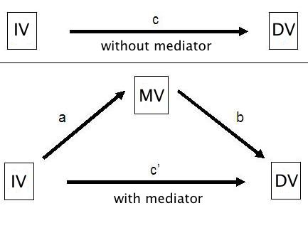
Mediator variables are variables that sit between the independent variable and dependent variable and mediate the effect of the IV on the DV. A model with one mediator is shown in the figure below.
The idea, in mediation analysis, is that some of the effect of the predictor variable, the IV, is transmitted to the DV through the mediator variable, the MV. And some of the effect of the IV passes directly to the DV. That portion of of the effect of the IV that passes through the MV is the indirect effect.
An earlier approach to multilevel mediation suggested by Krull & MacKinnon (2001) was method 1. This page will demonstrate an alternative approach given in the 2006 paper by Bauer, Preacher & Gil. This approach combines the dependent variable and the mediator into a single stacked response variable and runs one mixed model with indicator variables for the DV and mediator to obtain all of the values needed for the analysis.
We will begin by loading in a synthetic data set and reconfiguring it for our analysis. All of the variables in this example (id the cluster ID, x the predictor variable, m the mediator variable, and y the dependent variable) are at level 1 Here is how the first 16 observations look in the original dataset. The dataset is available as a comma separated values (CSV) file here: ml_sim.csv. Let’s start by reading in the data and looking at a few descriptive statistics.
get data
  /type=txt
  /file="D:\ml_sim.csv"
  /delimiters=","
  /firstcase=2
  /variables= id F2.0 x F m F y F.
execute.
dataset name ML_SIM.
compute fid = $casenum.
execute.

descriptives variables=id fid x m y
  /statistics=mean stddev range min max.
There are 100 level-2 units each with eight observations. fid is a row id, so when the data is not stacked, there is just 1 obsevation for each fid. Let’s look at the three models of a mediation analysis beginning with the model with just the IV.
mixed y with x
  /fixed =  x
  /random = intercept x | subject(id) covtype(un)
  /method = reml
  /print = solution testcov.
Next, comes the model with the mediator predicted by the IV.
mixed m with x
  /fixed =  x
  /random = intercept x | subject(id) covtype(un)
  /method = reml
  /print = solution testcov.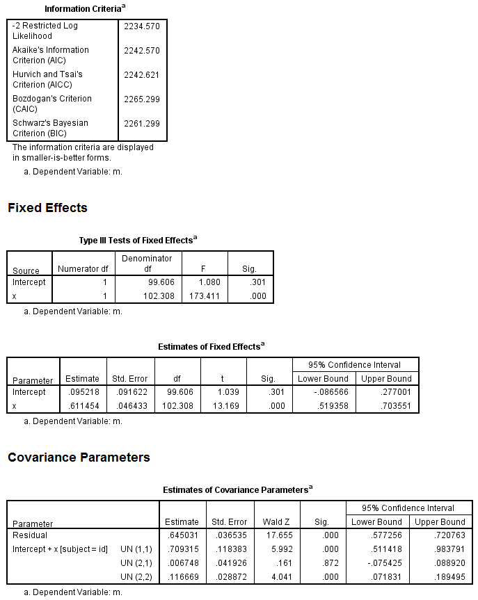
Finally, the model with both the IV and mediator predicting the DV.
mixed y with x m
  /fixed =  x m
  /random = intercept x m | subject(id) covtype(un)
  /method = reml
  /print = solution testcov.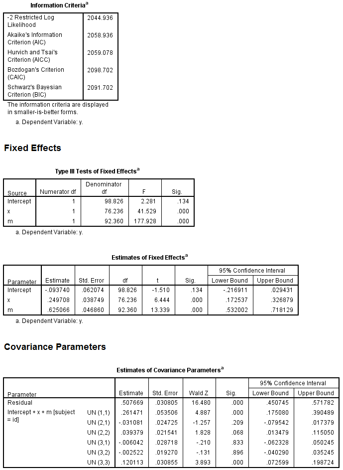
We see that the IV although still significant has been reduced from .69 to .25. Now, we need to restructure the data to stack y on m for each row and create indicator variables for both the mediator and the dependent variables. Here’s how we can do this (note that you will need to change the location of the new dataset to one on your computer).
vector variable = m to y.
loop sy = 1 to 2.
compute z = variable(sy).
xsave outfile 'D:\ml_simlong.sav'
  /drop y.
end loop.
execute.
get file'D:\ml_simlong.sav'.

compute sy = sy - 1.
compute sm = ~sy.
execute.
The new response variable is called z and has y stacked on m. We named the indicators for the mediator and the DV sm and sy respectively, to be consistent with Bauer et al (2006). We have also created a new m that contains the value for the mediator from each of the original observations.
Now we can run our mixed model for multilevel mediation using mixed. Notice that because we include the sm and sy indicators in the model that we need to use the NOINT option for the fixed effects (it is not automatically included for random effects, so there is no need to supress it). In addition to the random effects, we use a repeated subcommand to model the heterogeneity in residual variances for y and m (which are now stacked and just in the variable z.
mixed z with sm sy x m
  /fixed     = sm sm * x sy sy * m sy * x | noint
  /random = sm sm * x sy sy * m sy * x | subject(id) covtype(un)
  /repeated =  sm | subject(fid id) covtype(diagDIAG)
  /method = reml
  /print = g solution testcov covb.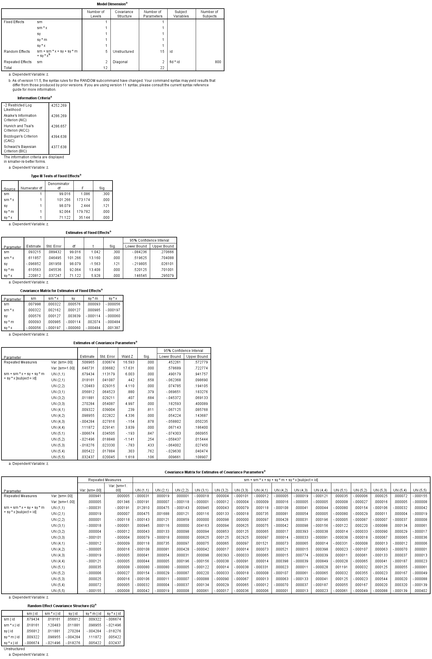
We now have access to all of the information needed to compute the average indirect effect and average total effect and their standard errors using the equations given in Bauer, et. al. (2006).
$$ ind = ab + \sigma_{a_{j}b_{j}} \quad (EQ:A11) $$ $$ Var(ind) = b^{2}\sigma^{2}_{\hat{a}} + a^{2}\sigma^{2}_{\hat{b}} + \sigma^{2}_{\hat{a}}\sigma^{2}_{\hat{b}} + 2ab\sigma_{\hat{a},\hat{b}} + (\sigma_{\hat{a},\hat{b}})^2 + \sigma^{2}_{\hat{\sigma}_{a_{j},b_{j}}} \quad (EQ:A14) $$
average total effect
$$ tot = ab + \sigma_{a_{j}b_{j}} + c’ \quad (EQ:A15) $$ $$ Var(ind) = b^{2}\sigma^{2}_{\hat{a}} + a^{2}\sigma^{2}_{\hat{b}} + 2ab\sigma_{\hat{a},\hat{b}} + 2b\sigma_{\hat{a},\hat{c}’} + 2a\sigma_{\hat{b},\hat{c}’} + \sigma^{2}_{\hat{\sigma}_{a_{j},b_{j}}} + \sigma^{2}_{\hat{c}’} + \sigma^{2}_{\hat{a}}\sigma^{2}_{\hat{b}} + (\sigma_{\hat{a},\hat{b}})^2 \quad (EQ:A18) $$
These formulae involve the fixed effects estimates, their variances and covariances, and variances and covariances from the random effects. Here are all the values
$$ a = 0.6119 \\ b = 0.6106 \\ c’ = 0.2208 \\ \sigma_{a_{j}b_{j}} = 0.09896 \\ \sigma^{2}_{\hat{a}} = 0.002162 \\ \sigma^{2}_{\hat{b}} = 0.002074 \\ \sigma_{\hat{a},\hat{b}} = 0.000985 \\ \sigma_{\hat{a},\hat{c}’} = -0.00020 \\ \sigma_{\hat{b},\hat{c}’} = -0.00048 \\ \sigma^{2}_{\hat{c}’} = 0.001387 \\ \sigma^{2}_{\hat{\sigma}_{a_{j},b_{j}}} = 0.02282^{2} $$
To calculate this, you just need a calculator. A simple way in SPSS is using SPSS’ matrix language, which essentially allows us to just declare the constants and write out the formulae.
matrix.
  compute a = 0.611857.
  compute b = 0.610563.
  compute rcov_ab = 0.098955.
  compute cprime = 0.220812.
  compute Va = 0.002162.
  compute Vb = 0.002074.
  compute Vcprime = 0.001387.
  compute cov_ab = 0.000985.
  compute cov_ac = -0.000197.
  compute cov_bc = -0.000484.
  compute Vcov_ab = 0.022822**2.

  compute ind_eff = a*b + rcov_ab.
  compute V_ind = a**2*Vb + b**2*Va + Va*Vb + 2*a*b*cov_ab + cov_ab**2 + Vcov_ab.
  compute test_ind = ind_eff/V_ind**.5.
  compute tot_eff = ind_eff + cprime.
  compute V_tot = b**2*Va + a**2*Vb + Va*Vb + 2*a*b*cov_ab + cov_ab**2 + Vcprime + 2*b*cov_ac + 2*a*cov_bc + Vcov_ab.
  compute test_tot = tot_eff/V_tot**.5.

  print ind_eff / FORMAT = F6.6 / title 'indirect effect'.
  print V_ind / FORMAT = F6.6 / title 'variance of indirect effect'.
  print test_ind / FORMAT = F6.6 / title 'significance test of indirect effect, test against standard normal'.
  print tot_eff / FORMAT = F6.6 / title 'total effect'.
  print V_tot / FORMAT = F6.6 / title 'variance of total effect'.
  print test_tot / FORMAT = F6.6 / title 'significance test of total effect, test against standard normal'.
end matrix.

Run MATRIX procedure:

indirect effect
 .47253

variance of indirect effect
 .00284

significance test of indirect effect, test against standard normal
 8.8597

total effect
 .69334

variance of total effect
 .00340

significance test of total effect, test against standard normal
 11.893

------ END MATRIX -----
Finally, note that it is possible to achieve the same effect as using the repeated subcommand using a second random subcommand. We add a random slope by fid to model the additional heterogeneity in outcomes. The residual variance is the residual variance of y, the residual variance plus the variance of the random slope is the residual variance for m. Note that this model takes some time to run.
mixed z with sm sy x m
  /fixed     = sm sm * x sy sy * m sy * x | noint
  /random = sm sm * x sy sy * m sy * x | subject(id) covtype(un)
  /random = sm | subject(fid)
  /method = reml
  /print = g solution testcov covb.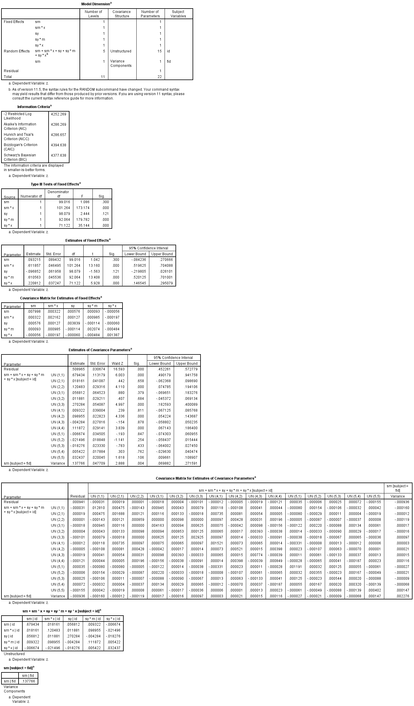
Note that .508965 + .137766 = 0.646731, the residual variance of m from our previous model, showing that these two approaches yield similar results, although the random slope approach is somewhat less direct.
References
- Bauer, D. J., Preacher, K. J. & Gil, K. M. (2006) Conceptualizing and testing random indirect effects and moderated mediation in multilevel models: New procedures and recommendations. Psychological Methods, 11(2), 142-163.
- Krull, J. L. & MacKinnon, D. P. (2001) Multilevel modeling of individual and group level mediated effects. Multivariate Behavioral Research, 36(2), 249-277.

