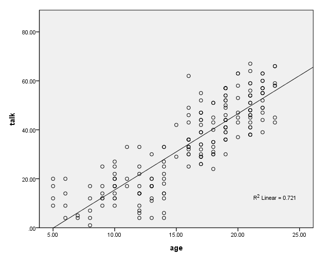
Say that you want to look at the relationship between how much a child talks on the phone and the age of the child. You get a random sample of 200 kids. You ask them how old they are and how many minutes they spend talking on the phone. Finally, you save the data as https://stats.idre.ucla.edu/wp-content/uploads/2016/02/talk.sav. You then make a scatterplot of the data as shown below.
GGRAPH
  /GRAPHDATASET NAME="iGraphDataset" VARIABLES= talk age
  /GRAPHSPEC SOURCE=INLINE INLINETEMPLATE=["<addFitLine  type='linear' target='pair'/> "].
BEGIN GPL
SOURCE: s=userSource( id( "iGraphDataset" ) )
DATA:talk=col( source(s), name( "talk" ) )
DATA: age=col( source(s), name( "age" ) )
GUIDE: axis( dim( 1 ), label( "age" ) )
GUIDE: axis( dim( 2 ), label( "talk" ) )
SCALE: linear( dim( 1 ), min( 5 ), max( 25 ) )
SCALE: linear( dim( 2 ), min( 0 ), max( 80 ) )
ELEMENT: point( position( ( age * talk ) ) )
END GPL.
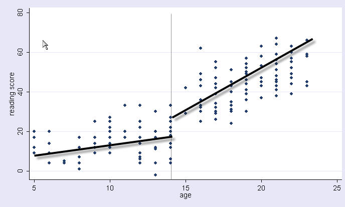
Thinking about this more, you decide that you think that the amount of time that kids talk on the phone changes dramatically at age 14, and that the slope might change at that age as well. You think that a piecewise regression might make more sense, where before age 14 there is an intercept and linear slope, and after age 14, there is a different intercept and different linear slope, kind of like pictured below with just freehand drawing of what the two regression lines might look like.
Try 1: Separate regressions
To investigate this, we can run two separate regressions, one for before age 14, and one for after age 14. We can compare the results of these two models.
* Before age 14.
compute before14 = (age < 14).
filter by before14.
regression /dep=talk /method=enter age.
filter off.
* At age 14 and after.
compute after14 = (age >= 14).
filter by after14.
regression /dep=talk /method=enter age.
filter off.
Note how the slopes do seem quite different for the two groups. However, the intercepts don’t make much sense, since they are the predicted time talking on the phone when one is 0 years old.
Try 2: Separate regression with age centered at 14
Let’s rescale (center) age by subtracting 14. Then, when age is 0, that really refers to being 14 years old.
* age14 subtracts 14 from age, so age is 0 when child is 14.
compute age14 = (age - 14).

* Now, rerun regression when child is below 14.
compute before14 = (age < 14).
filter by before14.
regression /dep=talk /method=enter age14.
filter off.

* Now, rerun regression when child is 14 years of age or older.
compute after14 = (age >= 14).
filter by after14.
regression /dep=talk /method=enter age14.
filter off.

Note how the slopes for the two groups stayed the same, but now the
intercepts (Constant) are the predicted talking time at age 14 for the two
groups. We can see that at age 14 there seems to be not only a change
in the slope (from .682 to 3.62) but also a jump in the intercept
(from 17.6 to 25.8). This suggest that at age 14, there is discontinuous
jump in time talking on the phone as well as a change in the slope as well.
However, this is merely suggestive; we should really test this in a combined
model.
Try 3: Combined model, coding for separate slope and intercept
We now combine the two models into a single model. To do this, we need to create some new variables.
- age1 is the age centered around age 14 but converted to 0s after age 14 (representing the effect of age for before 14 year olds).
- age2 is the age centered around age 14 but converted to 0s before 14 (representing the effect of age for after 14 year olds).
- int1 is 1 before age 14 (representing the intercept for before 14 year olds).
- int2 is 1 after age 14 (representing the intercept for after 14 year olds).
compute  age1 = (age - 14).
if (age >= 14) age1 = 0 .
compute  age2 = (age - 14).
if (age < 14) age2 = 0 .

compute  int1 = 1.
if (age >= 14) int1 = 0.
compute  int2 = 1.
if (age < 14)  int2 = 0.
execute.
That might have been confusing, so let us show what these variables look like in a table below. Note that we have a strange person who is 13.99 years old (very, very close to being 14, but not quite). This person will be helpful for seeing the effect of the jump from going from being under 14 to being 14.
* Check the coding.

* Save our data file so far.
save outfile = "c:datatalk2.sav".
execute.

* Collapse the data to make the coding easier to see.
aggregate
  /outfile=* mode = addvaraibles
  /break=age int1 int2 age1 age2
  /count=N.
list cases.
     age     int1     int2     age1     age2   count

     5.00     1.00      .00    -9.00      .00       4
     6.00     1.00      .00    -8.00      .00       4
     7.00     1.00      .00    -7.00      .00       2
     8.00     1.00      .00    -6.00      .00       5
     9.00     1.00      .00    -5.00      .00       6
    10.00     1.00      .00    -4.00      .00      13
    11.00     1.00      .00    -3.00      .00       3
    12.00     1.00      .00    -2.00      .00      13
    13.00     1.00      .00    -1.00      .00      11
    13.99     1.00      .00     -.01      .00       1
    14.00      .00     1.00      .00      .00      11
    15.00      .00     1.00      .00     1.00       2
    16.00      .00     1.00      .00     2.00      15
    17.00      .00     1.00      .00     3.00      20
    18.00      .00     1.00      .00     4.00      12
    19.00      .00     1.00      .00     5.00      25
    20.00      .00     1.00      .00     6.00       8
    21.00      .00     1.00      .00     7.00      22
    22.00      .00     1.00      .00     8.00      16
    23.00      .00     1.00      .00     9.00       7
Now we can go back to the talk2.sav data file before we did this collapsing.
get file = "c:datatalk2.sav".
Now we are ready to run our combined regression. We will put in the intercept for both groups, so we don’t need an intercept from SPSS so we use the origin option to put the regression through the origin (i.e., no intercept). This is necessary because our model has an implied constant, int1 plus int2 adds up to 1. Note that the r-square is not valid for this model and should not be reported.
* Run the regression, compare to try 2.
regression  /origin /dependent=talk
  /method=enter int1 int2 age1 age2
  /save=pred(yhat).
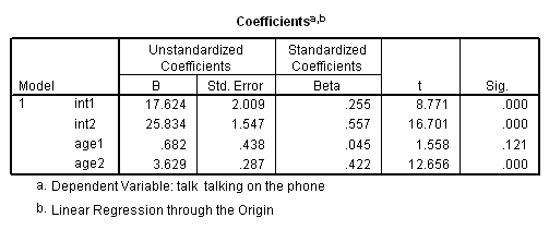
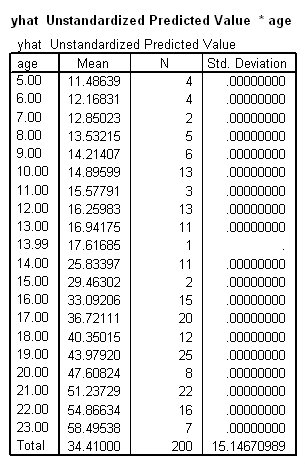
Now let’s obtain the predicted values (shown in the table below) and relate those to the meaning of the coefficients above.
- age1 is the slope when age is less than 14. For example, as you go from being age 5 to 6, phone talking goes from 11.48 to 12.17, and that equals .68 (with rounding).
- age2 is the slope when age is 14 or higher. For example, as you go from being age 15 to 16, phone talking goes from 29.46 to 33.09, and that equals 3.62 (with rounding).
- int1 is the predicted mean for someone who is just infinitely close to being 14 years old (but not quite 14). Note that when someone is 13.99 their predicted mean is very close to int1 (17.616 versus 17.624).
- int2 is the predicted mean for someone who just turned 14 years old, and note that 25.83 is the value for int2 and is the value for the predicted value at exactly age 14.
means tables=yhat by age.
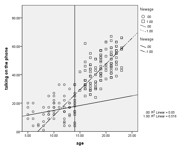
Below we show a graph of the results.
compute newage = 0.
if age ge 14 newage = 1.
exe.

GGRAPH
  /GRAPHDATASET NAME="iGraphDataset" VARIABLES= talk age newage
  /GRAPHSPEC SOURCE=INLINE EDITABLE=YES
      INLINETEMPLATE=["<addFitLine  type='linear' target='subgroup'/>" ].
BEGIN GPL
SOURCE: s=userSource( id( "iGraphDataset" ) )
DATA: talk=col( source(s), name( "talk" ) )
DATA: age=col( source(s), name( "age" ) )
DATA: newage=col( source(s), name( "newage" ), unit.category()  )
GUIDE: axis( dim( 1 ), label( "age" ) )
GUIDE: axis( dim( 2 ), label( "talking on the phone" ) )
GUIDE: legend( aesthetic( aesthetic.shape.interior ), label( "newage" ) )
SCALE: linear( dim( 1 ), min( 5 ), max( 25 ) )
SCALE: linear( dim( 2 ), min( 0 ), max( 80 ) )
GUIDE: form.line(position(14, *))
ELEMENT: point( position( age * talk ), shape.interior(newage) )
ELEMENT: line( position( smooth.linear(age * talk ) ), shape.interior( newage) )
GUIDE: legend(aesthetic(aesthetic.shape), label("Newage") )
END GPL.
You might want to test whether the difference in the intercepts is 0 or whether the change in the slopes is different from 0. The next section shows how we can do this.
Try 4: Alternate coding, coding to compare intercepts and slopes
This is another way you can code this model. Note that we include age14 and age2 for the two terms for age, and include the intercept (by not excluding it) and int2 to represent the intercept values. With this coding, age2 and int2 represent the change in slope and intercept from being less than 14 to being 14 and older.
regression
/dependent=talk
/method=enter age14 age2 int2
/save=pred(yhat2).
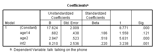
Using this coding scheme, here is the meaning of the coefficients.
- age14 is the slope when age is less than 14.
- age2 is the change in the slope as a result of becoming age 14 or higher (as compared to being less than 14).
- (Constant) is the predicted mean for someone who is just infinitely close to being 14 years old (but not quite 14).
- int2 is the predicted mean for someone who just turned 14 years old minus the predicted mean for someone who is infinitely close to being 14 years old (the jump that occurs at age 14).
As you can see, the coefficients for age2 and int2 now focus on the change that results from becoming 14 years old.
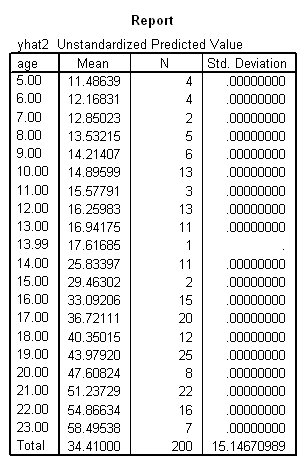
Below we compute the predicted values calling them yhat2. Note how the predicted values are the same for this model and the prior model, because the models are essentially the same, they are just parameterized differently.
means tables=yhat2 by age.
Summary
This brief FAQ compared different ways of creating piecewise regression models. All of these models are equivalent, just parameterized differently. They all generate the exact predicted values. The differences in parameterization are merely a rescrambling of the intercepts and slopes for the two segments of the regression model. You can choose the coding strategy that you like best, although it is often useful to use both schemes.

