Sometimes, a data set may have "holes" in them, i.e., missing values. Some statistical procedures such as regression analysis will not work as well, or at all on data set with missing values. The observations with missing values have to be either deleted or the missing values have to be substituted in order for a statistical procedure to produce meaningful results. Thus we may want to know the number of missing values and the distribution of those missing values so we have a better idea on what to do with the observations with missing values. Let’s look at the following data set.
 LANDVAL  IMPROVAL    TOTVAL  SALEPRIC SALTOAPR

   30000     64831     94831    118500   1.25
 30000     50765     80765     93900    .
   46651     18573     65224         .   1.16
   45990     91402         .    184000   1.34
   42394         .     40575    168000   1.43
       .      3351     51102    169000   1.12
   63596      2182     65778         .   1.26
   56658     53806     10464    255000   1.21
   51428     72451         .         .   1.18
   93200         .      4321    422000   1.04
   76125     78172     54297    290000   1.14
       .     61934     16294    237000   1.10
   65376     34458         .    286500   1.43
  42400         .     57446         .    .
   40800     92606     33406    168000   1.26
1. Number of missing values vs. number of non missing values
The first thing we are going to look at is what the variables are that have a lot of missing values. We just use the command frequencies with option /format=notable.
FREQUENCIES VARIABLES=landval improval totval salepric saltoapr
  /FORMAT=NOTABLE
  /ORDER= ANALYSIS .

So we know the number of missing values in each variable. For instance, variable salepric has four and saltoapr has two missing values. This will help us to identify variables that may have a large number of missing values and perhaps we may want exclude those from analysis.
2. Number of missing values in each observation and its distribution
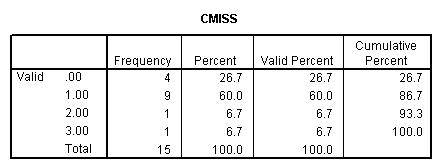
We can also look at the distribution of missing values across observations. For example we use command count to create a new variable cmiss counting the number of missing values across each observation. Looking at its frequency table we know that there are four observations with no missing values, nine observations with one missing values, one observation with two missing values and one observation with three missing values. If we are willing to substitute one missing value per observation, we will be able to reclaim nine observations back to get a valid data set that is 13/15=87% of the size of the original one.
COUNT
  cmiss = landval improval totval salepric saltoapr  (MISSING).

FREQUENCIES VARIABLES=cmiss
  /ORDER=  ANALYSIS .

3. Distribution of missing values
We can also look at the patterns of missing values. We can recode each variable into a dummy variable such that 1 is missing and 0 is nonmissing. Then we use the aggregate command to compute the frequency for each pattern of missing data.
RECODE
  landval improval totval salepric saltoapr
  (MISSING=1)  (ELSE=0)  INTO  land1  impr1  totv1  sale1  salt1 .
EXECUTE .
AGGREGATE
  /OUTFILE='AGGR.SAV'
  /BREAK=land1 impr1 totv1 sale1 salt1
  /N_BREAK=N.
File AGGR.SAV has the following variables and observations.LAND1 IMPR1 TOTV1 SALE1 SALT1 N_BREAK .00 .00 .00 .00 .00 4 .00 .00 .00 .00 1.00 1 .00 .00 .00 1.00 .00 2 .00 .00 1.00 .00 .00 2 .00 .00 1.00 1.00 .00 1 .00 1.00 .00 .00 .00 2 .00 1.00 .00 1.00 1.00 1 1.00 .00 .00 .00 .00 2
Now we see that there are four observations with no missing values, one observation with one missing value in variable saltoapr, two observations with missing value in variable salepric and one observation with missing value in both variable totval and salepric, etc. If we want to delete some observations from the original data set, we have a better idea now on which observation to delete, e.g. the observation corresponding to the 7th row above.
