Suppose we have an ANOVA model, and we would like to compare means between one group and another group. This is commonly done with the lmatrix subcommand in SPSS. Let’s look at a simple example using a data set called https://stats.idre.ucla.edu/wp-content/uploads/2016/02/elemapi2.sav . The dependent variable is the school’s API index (a continuous variable). The variables mealcat and collcat are categorical variables, both with three levels. These will be used as the predictor variables. This model is shown below. We have included the emmeans subcommand to get the expected means for each group. This can be helpful if you want to calculate the contrast estimate by hand.
glm api00 by collcat mealcat
/design = collcat mealcat collcat*mealcat
/emmeans = tables (collcat*mealcat).
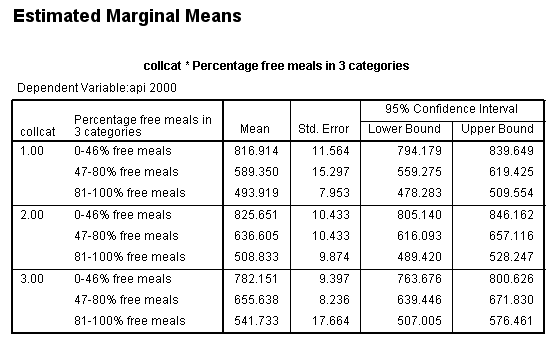
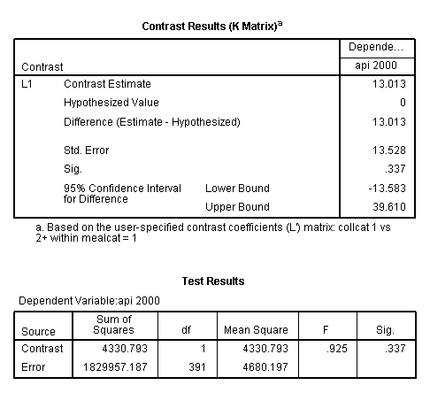
Let’s say that we want to look at a simple comparison of group 1 versus 2 and above of collcat when mealcat = 1. One way of doing this using the glm command with lmatrix subcommand. We use the test(lmatrix) option on the print subcommand to have SPSS print out the contrast coefficients that are applied to each group.
glm api00 by collcat mealcat
/design = collcat mealcat collcat*mealcat
/print = test(lmatrix)
/lmatrix 'collcat 1 vs 2+ within mealcat = 1'
              collcat 1 -.5 -.5
              collcat*mealcat 1   0   0
		             -.5  0   0
		             -.5  0   0.
While this lmatrix subcommand will run the analysis we want, it is a little difficult to write. Another way of accomplishing the same thing is to use a cell means model. A cell means model estimates only one parameter for each cell and sets the intercept to 0. In general, the cell means model is not used to produce an overall test of model fit, but it is often used to write simpler lmatrix subcommands. So, in practice, we need to write the glm code twice, once for the model fit and the second time for the estimates. In the code shown below, the first glm command is for model fit and the second one with the lmatrix subcommand is used to estimate the simple comparison.
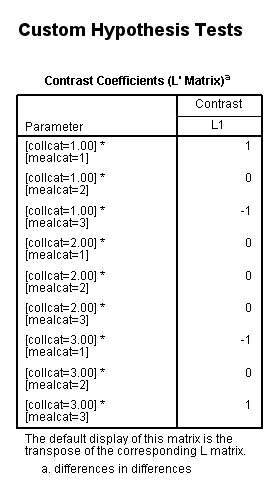
In the second call to glm, which is a cell means model, the main effects are omitted; only the interaction is included in the model. We use the exclude option on the intercept subcommand to specify that we are not going to estimate the intercept; therefore, we will estimate one parameter per cell. We use the test(lmatrix) option on the print subcommand to show us the contrast codes that were used. This is a useful way to be sure that the contrast codings were assigned as you intended.
* estimating the overall model.
glm api00 by collcat mealcat
/design = collcat mealcat collcat*mealcat.
* estimating the cell means model to get the desired estimate. glm api00 by collcat mealcat /design = collcat mealcat collcat*mealcat /print = test(lmatrix) /lmatrix 'collcat 1 vs 2+ within mealcat = 1' collcat 1 -.5 -.5 collcat*mealcat 1 0 0 -.5 0 0 -.5 0 0.
Notice that the order of categorical variables on the lmatrix subcommand decides which variable is the row variable and which is the column variable. For example, in the code above, collcat will be the row variable and mealcat will be the column variable. Therefore, the simple comparison we are interested in can be formulated as shown in the following table. Writing the numbers in the table one row at a time, we can write our lmatrix subcommand as:
  lmatrix 'simple comparison'
              collcat*mealcat 1 0 0 -.5 0 0 -.5 0 0
| collcat /mealcat | mealcat = 1 | mealcat = 2 | mealcat = 3 |
| collcat = 1 | 1 | 0 | 0 |
| collcat =2 | -.5 | 0 | 0 |
| collcat = 3 | -.5 | 0 | 0 |
If we switch the order of variables on the lmatrix subcommand, we will have to rewrite our
terms accordingly. For example, we can rewrite the above lmatrix
subcommand as the
following; it produces exactly the same result from the lmatrix
subcommand, since the corresponding table is simply being transposed.
| mealcat /collcat |
collcat = 1 | collcat =2 | collcat=3 |
| mealcat = 1 | 1 | -.5 | -.5 |
| mealcat = 2 | 0 | 0 | 0 |
| mealcat = 3 | 0 | 0 | 0 |
Let’s run the analysis model. Notice that both collcat and the collcat*mealcat interaction need to be specified on the lmatrix subcommand.
glm api00 by collcat mealcat
/design = collcat mealcat collcat*mealcat
/print = test(lmatrix)
/lmatrix 'collcat 1 vs 2+ within mealcat = 1'
              collcat 1 -.5 -.5
              collcat*mealcat 1   0   0
		             -.5  0   0
		             -.5  0   0.
< some output omitted >
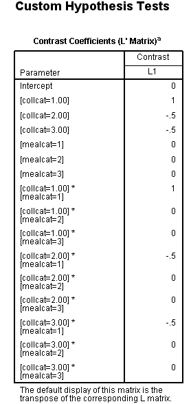
This simple comparison is not statistically significant (t = 0.96, p = 0.3367).
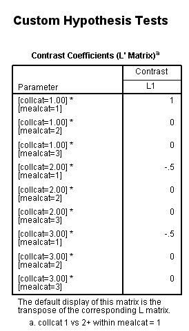
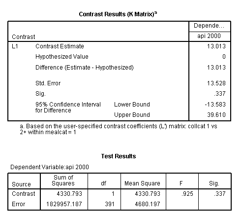
Now let’s run the cell means model. Notice that only the interaction term is used on the design and the lmatrix subcommands.
glm api00 by collcat mealcat
/design = collcat*mealcat
/intercept = exclude
/print = test(lmatrix)
/lmatrix = 'collcat 1 vs 2+ within mealcat = 1'
               collcat*mealcat 1 0 0 -.5 0 0 -.5 0 0.
< some output omitted >
Brief summary
- A cell means model is used only for the purpose of making the contrast on a lmatrix subcommand easier to write. The only part of the output that is considered is the part related to the contrast estimate (this is usually found at the bottom of the output).
- Writing the lmatrix subcommand with a cell means model is easier because it includes only one vector (for highest-order interaction). Using the analysis model, the lmatrix subcommand for the same contrast may contain multiple vectors and/or matrices and is therefore more difficult to specify correctly.
- The cell means model approach can be used with models that include three-way or higher interactions. Only the highest-order interaction is included on the design subcommand, and only this term is used on the lmatrix subcommandt.
- A cell means model can be used with other procedures, such as mixed.
Example 2
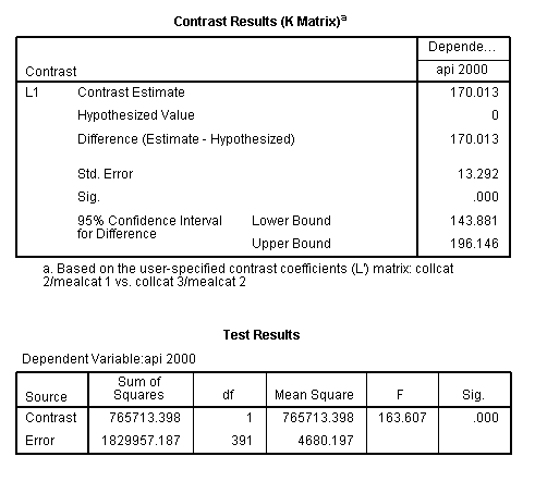
In our second example, we will compare the means between two cells in the design. Specifically, we will compare collcat=2 at mealcat=1 to collcat=3 at mealcat=2.
| collcat /mealcat | mealcat = 1 | mealcat = 2 | mealcat = 3 |
| collcat = 1 | 0 | 0 | 0 |
| collcat =2 | 1 | 0 | 0 |
| collcat = 3 | 0 | -1 | 0 |
The lmatrix subcommand for this comparison is shown below.
glm api00 by collcat mealcat
/design = collcat mealcat collcat*mealcat
/print = test(lmatrix)
/lmatrix = 'collcat 2/mealcat 1 vs. collcat 3/mealcat 2'
              collcat 0 1 -1
			  mealcat 1 -1 0
              collcat*mealcat 0 0 0
		             1   0  0
		             0  -1  0.
< some output omitted >
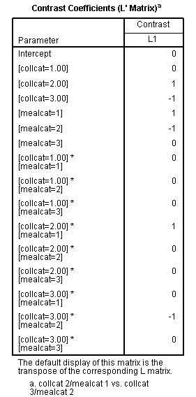
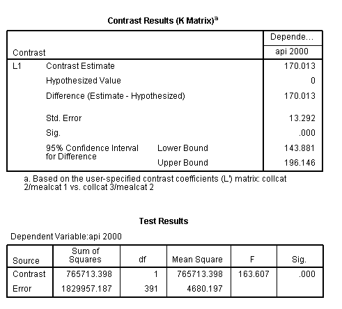
This comparison is statistically significant (t = 12.79, p < .0001).
Using the cell means model, the lmatrix subcommand is constructed as shown below.
glm api00 by collcat mealcat
/design = collcat*mealcat
/intercept = exclude
/print = test(lmatrix)
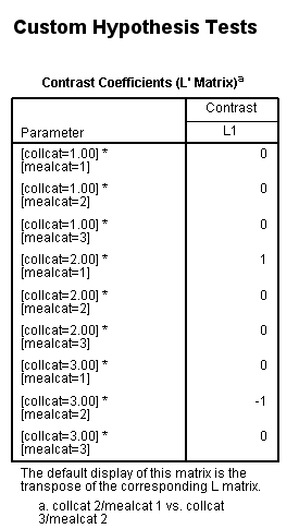
/lmatrix = 'collcat 2/mealcat 1 vs. collcat 3/mealcat 2'
collcat*mealcat 0 0 0 1 0 0 0 -1 0.
< some output omitted >
Example 3
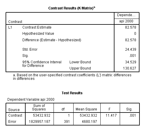
In our last example, we will look at a difference in differences. We will take the difference between the difference of ([collcat=1 and mealcat=1] and [collcat=1 and mealcat=3]) and ([collcat=3 and mealcat=1] and [collcat=3 and mealcat=3]).
Remember that a little bit of math needs to be done to get the correct signs of the contrast coefficients: (collcat=1/mealcat=1 – collcat=1/mealcat=3) – (collcat=3/mealcat=1 – collcat=3/mealcat=3) = collcat=1/mealcat=1 – collcat=1/mealcat=3 – collcat=3/mealcat=1 + collcat=3/mealcat=3.
| collcat /mealcat | mealcat = 1 | mealcat = 2 | mealcat = 3 |
| collcat = 1 | 1 | 0 | -1 |
| collcat =2 | 0 | 0 | 0 |
| collcat = 3 | -1 | 0 | 1 |
glm api00 by collcat mealcat
/design = collcat mealcat collcat*mealcat
/print = test(lmatrix)
/lmatrix = 'differences in differences'
               collcat*mealcat 1 0 -1
		              0 0 0
		             -1 0 1.
< some output omitted >
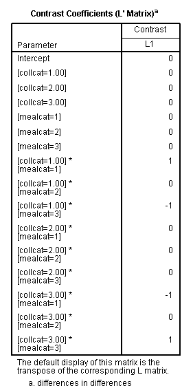
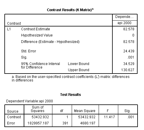
The comparison is statistically significant (t = 3.38, p = .0008).
Here is the lmatrix subcommand using the cell means model.
glm api00 by collcat mealcat
/design = collcat*mealcat
/intercept = exclude
/print = test(lmatrix)
/lmatrix = 'differences in differences'
               collcat*mealcat 1 0 -1 0 0 0 -1 0 1.
< some output omitted >
