You can use multiple lmatrix subcommands to explore the interaction of three categorical variables in ANOVA. If you are not familiar with three-way interactions in ANOVA, please see our general FAQ on understanding three-way interactions in ANOVA. In short, a three-way interaction means that there is a two-way interaction that varies across levels of a third variable. Say, for example, that a b*c interaction differs across various levels of factor a.
One way of analyzing the three-way interaction is through the use of tests of simple main-effects, e.g., the effect of one variable (or set of variables) across the levels of another variable.
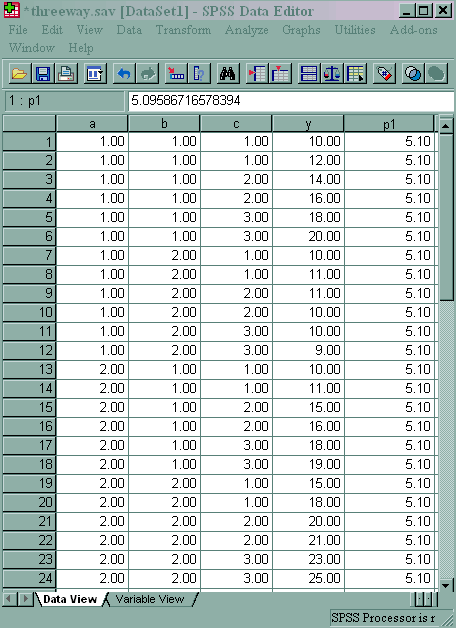
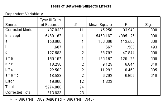
We will use a small artificial dataset called threeway that has a statistically significant three-way interaction to illustrate the process. In our example data set, variables a, b and c are categorical. The techniques shown on this page can be generalized to situations in which one or more variables are continuous, but the more continuous variables that are involved in the interaction, the more complicated things get.
The results (shown below) indicate that the b*c interaction is statistically significant at a=1 but not at a=2. Because of this, the second two lmatrix subcommands are needed; these show the effect of c at a=1 at both levels of b.
After we look at the results, we will look at the coding used.
glm y by a b c
  /design = a b c a*b a*c b*c a*b*c
  /lmatrix 'b*c at a=1' b*c 1 0 -1 -1  0 1 a*b*c 1 0 -1 -1  0 1 0 0 0 0 0 0;
                        b*c 0 1 -1  0 -1 1 a*b*c 0 1 -1  0 -1 1 0 0 0 0 0 0

  /lmatrix 'b*c at a=2' b*c 1 0 -1 -1  0 1 a*b*c 0 0 0 0 0 0 1 0 -1 -1  0 1;
                        b*c 0 1 -1  0 -1 1 a*b*c 0 0 0 0 0 0 0 1 -1  0 -1 1

  /lmatrix 'c at a=1 & b=1' c 1 0 -1 a*c 1 0 -1 0 0 0 b*c 1 0 -1 0 0 0 a*b*c 1 0 -1  0 0 0 0 0 0 0 0 0;
                            c 0 1 -1 a*c 0 1 -1 0 0 0 b*c 0 1 -1 0 0 0 a*b*c 0 1 -1  0 0 0 0 0 0 0 0 0

  /lmatrix 'c at a=1 & b=2' c 1 0 -1 a*c 1 0 -1 0 0 0 b*c 0 0 0 1 0 -1 a*b*c 0 0 0 1 0 -1 0 0 0 0 0 0;
                            c 0 1 -1 a*c 0 1 -1 0 0 0 b*c 0 0 0 0 1 -1 a*b*c 0 0 0 0 1 -1 0 0 0 0 0 0.
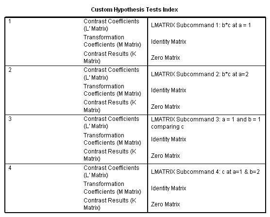
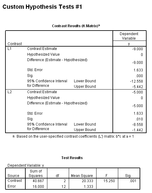
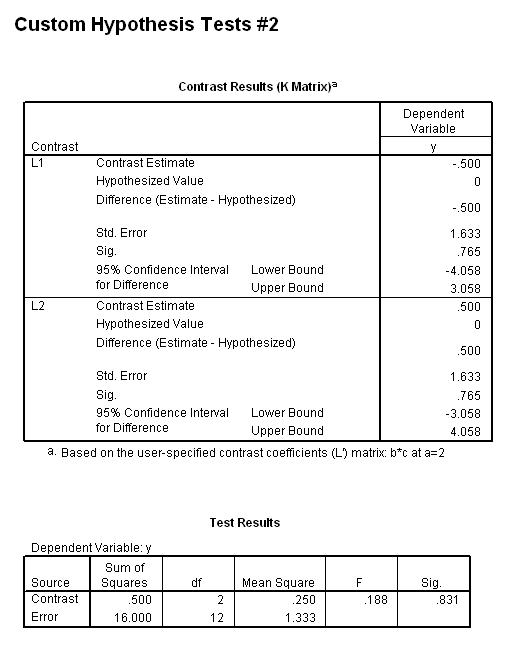
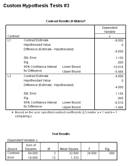
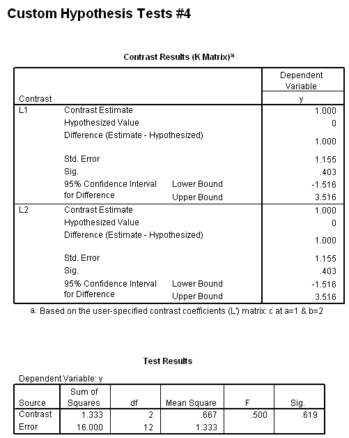
In the first lmatrix subcommand, we are interested in the b*c interaction at a=1. The b*c interaction has 2 degrees of freedom ( (2-1)*(3-1) = 2 ). To indicate this, we use a semicolon to separate the two parts. Also, because we have included the two-way interaction, we also need to include the three-way interaction. In the second lmatrix subcommand, we are looking at the b*c interaction at a=2. Realistically, we wouldn’t know to to include the third and fourth lmatrix subcommands until we had run the first two and seen the results. To save space, we have included these two lmatrix subcommands, which investigate c at a=1 and both levels of b.
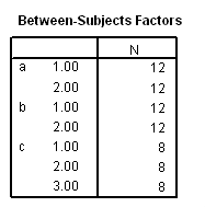
Let’s look a little closer at the coding of the variables on the lmatrix subcommands. First, we need to remember that the variable a has two levels, b has two levels, and c has three levels. The coding (which is effect coding) is for each cell produced by the crossing of the categorical predictor variables. This is perhaps best understood as the "differences of differences" approach. (For more information, please see Multiple Regression: Testing and Interpreting Interactions by Leona S. Aiken and Steven G. West).
glm y by a b c
  /design = a b c a*b a*c b*c a*b*c
  /lmatrix 'b*c at a=1' b*c 1 0 -1 -1  0 1 a*b*c 1 0 -1 -1  0 1 0 0 0 0 0 0;
                        b*c 0 1 -1  0 -1 1 a*b*c 0 1 -1  0 -1 1 0 0 0 0 0 0

  /lmatrix 'b*c at a=2' b*c 1 0 -1 -1  0 1 a*b*c 0 0 0 0 0 0 1 0 -1 -1  0 1;
                        b*c 0 1 -1  0 -1 1 a*b*c 0 0 0 0 0 0 0 1 -1  0 -1 1

  /lmatrix 'c at a=1 & b=1' c 1 0 -1 a*c 1 0 -1 0 0 0 b*c 1 0 -1 0 0 0 a*b*c 1 0 -1 0 0 0 0 0 0 0 0 0;
                            c 0 1 -1 a*c 0 1 -1 0 0 0 b*c 0 1 -1 0 0 0 a*b*c 0 1 -1 0 0 0 0 0 0 0 0 0

  /lmatrix 'c at a=1 & b=2' c 1 0 -1 a*c 1 0 -1 0 0 0 b*c 0 0 0 1 0 -1 a*b*c 0 0 0 1 0 -1 0 0 0 0 0 0;
                            c 0 1 -1 a*c 0 1 -1 0 0 0 b*c 0 0 0 0 1 -1 a*b*c 0 0 0 0 1 -1 0 0 0 0 0 0.
The first lmatrix subcommand
Let’s take the first line of the first lmatrix subcommand as an example. We have the b*c interaction at a=1, and we are comparing c1 to c3. In other words, c3 is our reference group. Picking c3 as our reference group is somewhat arbitrary; we could have used c1 or c2. The "differences of differences" approach means that we are going to take the difference of c1 and c3 at b=1, and the difference of c1 and c3 at b=2, and then take the difference of those two differences. In the table below, we have six cells (because 2 levels of b times 3 levels of c equals 6). We have called the cells msubscript, so that we can do some symbolic math.
a=1
| c1 | c2 | c3 | |
| b=1 | m11 | m12 | m13 |
| b=2 | m21 | m22 | m23 |
(m11 – m13) – (m21 – m23)
(1 0 -1) – (1 0 -1) = 1 0 -1 -1 0 1
Notice that 1 0 -1 -1 0 1 are the first six entries in the first line of the first lmatrix subcommand.
Now let’s look at the second part, the a*b*c interaction. The first six numbers are for a=1, and the second six are for a=2. Because we are only looking at a=1 in this analysis, all of the values for a=2 are 0. The values for a=1 are the same as those for the b*c interaction.
Here is another way of thinking about the first line of the first lmatrix subcommand:
/lmatrix 'b*c at a=1' b*c 1 0 -1 -1 0 1 a*b*c 1 0 -1 -1 0 1 0 0 0 0 0 0;
Yellow: b=1, comparing c1 with c3
Orange: b=2, comparing c1 with c3
Green: a=1 and b=1, comparing c1 with c3
Blue: a=1 and b=2, comparing c1 with c3
Pink: a=2 and b=1, these are all 0s because we are looking only at a=1
Purple: a=2 and b=2, these are all 0s because we are looking only at a=1
The second line of the first lmatrix subcommand is very similar to the first, except that it is for c2 versus c3. So, we have
(m12 – m13) – (m22 – m23)
(0 1 -1) – (0 1 -1) = 0 1 -1 0 -1 1
  /lmatrix 'b*c at a=1' b*c 1 0 -1 -1  0 1 a*b*c 1 0 -1 -1  0 1 0 0 0 0 0 0;
                        b*c 0 1 -1  0 -1 1 a*b*c 0 1 -1  0 -1 1 0 0 0 0 0 0
Yellow: b=1, comparing c2 with c3
Orange: b=2, comparing c2 with c3
Green: a=1 and b=1, comparing c2 with c3
Blue: a=1 and b=2, comparing c2 with c3
Pink: a=2 and b=1, these are all 0s because we are looking only at a=1
Purple: a=2 and b=2, these are all 0s because we are looking only at a=1
The second lmatrix subcommand
The second lmatrix subcommand looks at the b*c interaction at a=2. It is the same as the first, except in the part for the a*b*c interaction. Here, the first six 0s are for a=1, which we are not considering in this lmatrix subcommand. The same coding used in the first lmatrix subcommand is simply shifted to the a=2 part of the code.
The third lmatrix subcommand
  /lmatrix 'c at a=1 & b=1' c 1 0 -1 a*c 1 0 -1 0 0 0 b*c 1 0 -1 0 0 0 a*b*c 1 0 -1 0 0 0 0 0 0 0 0 0;
                            c 0 1 -1 a*c 0 1 -1 0 0 0 b*c 0 1 -1 0 0 0 a*b*c 0 1 -1 0 0 0 0 0 0 0 0 0
By now, the coding for c, the first part of the lmatrix subcommand, should be familiar. In this first line, we are comparing c1 with c3.
a=1
| c1 | c2 | c3 | |
| b=1 | m11 | m12 | m13 |
| b=2 | m21 | m22 | m23 |
(m11 – m13) – (m21 – m23)
(1 0 -1) – (1 0 -1) = 1 0 -1 -1 0 1
Red: comparing c1 with c3
Light blue: a=1, comparing c1 and c3
Dark green: a=2, these are all 0 because we are looking at a=1
Yellow: b=1, comparing c1 with c3
Orange: b=2, these are all 0 because we are looking at b=1
Light green: a=1, b=1, comparing c1 with c3
Dark blue: a=1, b=2, these are all 0 because we are looking at b=1
Pink: a=2, b=1, these are all 0 because we are looking at a=1
Purple: a=2, b=2, these are all 0 because we are looking at a=1 and b=1
The second line of the third lmatrix subcommand is very similar to the first line, except that it compares c2 to c3.
  /lmatrix 'c at a=1 & b=1' c 1 0 -1 a*c 1 0 -1 0 0 0 b*c 1 0 -1 0 0 0 a*b*c 1 0 -1 0 0 0 0 0 0 0 0 0;
                            c 0 1 -1 a*c 0 1 -1 0 0 0 b*c 0 1 -1 0 0 0 a*b*c 0 1 -1 0 0 0 0 0 0 0 0 0
Light blue: a=1, comparing c2 and c3
Dark green: a=2, these are all 0 because we are looking at a=1
Yellow: b=1, comparing c2 with c3
Orange: b=2, these are all 0 because we are looking at b=1
Light green: a=1, b=1, comparing c2 with c3
Dark blue: a=1, b=2, these are all 0 because we are looking at b=1
Pink: a=2, b=1, these are all 0 because we are looking at a=1
Purple: a=2, b=2, these are all 0 because we are looking at a=1 and b=1
The fourth lmatrix subcommand
The fourth lmatrix subcommand is the same as the third, except we are now looking at b=2. Hence, we have 0s for the b=1 part of the code and the comparisons of the different levels of c in the b=2 part of the code.
  /lmatrix 'c at a=1 & b=2' c 1 0 -1 a*c 1 0 -1 0 0 0 b*c 0 0 0 1 0 -1 a*b*c 0 0 0 1 0 -1 0 0 0 0 0 0;
                            c 0 1 -1 a*c 0 1 -1 0 0 0 b*c 0 0 0 0 1 -1 a*b*c 0 0 0 0 1 -1 0 0 0 0 0 0.
Correcting for multiple tests
We should note that although a p-value is given for each of the four F-tests, it is not corrected for the multiple tests. There are at least four different methods of determining the critical value of tests of simple main-effects. There is a method related to Dunn’s multiple comparisons, a method attributed to Marascuilo and Levin, a method called the simultaneous test procedure (very conservative and related to the Scheffé post-hoc test) and a per family error rate method. We will demonstrate the per family error rate method, but you should look up the other methods in a good ANOVA book, such as Kirk (1995), to decide which approach is best for your situation.
Let’s take the first two tests, comparing b*c at a=1 and at a=2 as an example. The values for the F-tests were 15.25 and .188, respectively. We divide our alpha level, 0.05, by 2 because we are doing two tests of simple main-effects, so our new value of alpha is .025. The idf function requires us to provide 1 – alpha, so we have 1 – .025 = .975.
compute p1 = idf.f(.975, 2, 12).
exe.
As you can see, p1 is approximately 5.10. This indicates that the b*c interaction is statistically significant at a=1 but not at a=2.
References
Kirk, Roger E. (1995) Experimental Design: Procedures for the Behavioral Sciences, Third Edition. Monterey, California: Brooks/Cole Publishing.
Aiken, Leona S., and West, Stephen G. (1996) Multiple Regression: Testing and Interpreting Interactions. Thousand Oaks, California: Sage Publishing.

