SPSS has several commands that allow users to generate new variables using functions. Among these are compute, create and shift values. Below we will show some of the similarities and differences between these commands, so that you can decide which command best suits your needs.
All of our examples will use the hsb2.sav dataset. Because these three commands only have two functions in common, we will focus on these functions, lag and lead. However, the behavior of the command in the different situations will be the same regardless of the function used.
Introduction to the three commands
The compute command is perhaps the most commonly used command to generate new variables. There are many functions that can be used with the compute command, including arithmetic, statistical, random number, string and date/time functions. The compute command does not produce output or variable labels when it generates a new variable. Technically, compute is not a command, but rather a transformation. This means that, unlike a command such as create or shift values, compute does not read the active dataset. Rather, it is stored, pending execution with the next command that reads the active dataset. This is why the execute command is often used immediately after compute, but it is not necessary after create or shift values.
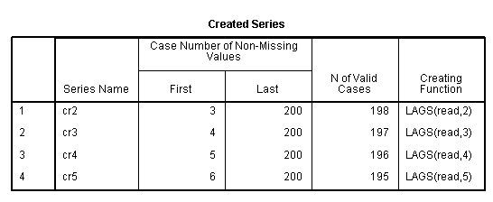
The create command is often used with time-series data and has about a dozen functions. The create command produces some output when it generate new variables, and it labels those variables. For more information on the create command, please see What kinds of new variables can I make with the create command? .
The shift values command was added in SPSS version 17 and has only three functions: lag, lead and shift. If a positive value is given with the shift function, it acts like lead; if a negative value is given, it acts like lag. The shift values command does not produce output when it generates new variables, but those variables are labeled.
Making multiple variables in a single call to the command
Both the create and shift values commands can generate multiple variables in a single call to the command; the compute command can not. Note that in the shift values command, the variable subcommand cannot be shortened to var.
create cr1 = lag(read, 1).create cr2 to cr5 = lag(read, 2, 5).
shift values variable = read result=sv1 lead = 1.
shift values variable = read result=sv2 lead = 2
 /variable = read result=sv3 lag = 2
 /variable = read result=sv4 lag = 3
 /variable = read result=sv5 lag = 4.
User-defined missing
We do not have any user-defined missing values in our dataset, so we will make some for this example.
if science gt 70 science = -9999.
missing values science (-9999).
exe.
The compute and create commands transform the user-defined missing into system missing values; only the shift values command retains the user-defined missing.
compute x41 = lag(science, 1).
create x42 = lag(science, 1).
shift values variable = science result = x43 lag = 1.
Execute
There are two types of commands in SPSS: transformations and procedures. Transformations include compute, if, recode and count. Transformations do not force SPSS to read through the dataset, and so nothing happens until a procedure forces SPSS to read through the dataset. For example, if you run a compute command by itself, you will see a message in the lower left corner of the window a message that says "Transformations pending".
Procedures require SPSS to read through the dataset. The execute command is an "empty" procedure; all it does is force SPSS to read through the dataset. The commands create and shift values are procedures, so the execute command is not needed after them. However, because the compute command is a transformation, some procedure, often execute, must follow to allow compute to generate the new variable. The execute command is often shortened to exe. Both sets of commands below will generate the variables cr7, sv7 and co7.
create cr7 = lag(write, 1).
shift values variable = write result = sv7 lag = 1.
compute co7 = lag(write, 1).
exe.
compute co7 = lag(write, 1). create cr7 = lag(write, 1). shift values variable = write result = sv7 lag = 1.
Temporary
The temporary command allows transformations to be in effect for the next procedure. The compute command cannot be used with the lag function after temporary, so we will generate a new variable by simply adding 1 to the variable write. As expected, the variable co8 is available for use in the first call to the descriptives command (shortened to desc) but not the second call. The shift values command does not respect the temporary command; hence, the variable sv8 is available for use in both desc calls. The create command does not respect the temporary command either. However, it does not generate the new variable because of the temporary command, as the warning message indicates.
temporary.
compute co8 = write + 1.
desc var = co8.

	desc var = co8.

temporary.
shift values variable = write result = sv8 lag= 1.
desc var = sv8.

	desc var = sv8.

temporary.
create cr8 = lag(write, 1).
desc var = cr8.

	desc var = cr8.
Filter
The compute, create and shift values commands do not respect the filter command; all cases (except the first case, of course) are populated with the lagged value.
sort cases by female.
filter by female.
compute co9 = lag(write, 1).
create cr9 = lag(write, 1).
shift values variable = write result = sv9 lag = 1.
filter off.
list female write co9 cr9 sv9
/cases from 1 to 92.
female write co9 cr9 sv9 .00 52.00 . . . .00 33.00 52.00 52.00 52.00 .00 44.00 33.00 33.00 33.00 < some output omitted > .00 49.00 62.00 62.00 62.00 1.00 59.00 49.00 49.00 49.00 Number of cases read: 92 Number of cases listed: 92
Split file
The create and shift values commands respect the split file command. However, compute does not. This is because the create and shift values commands read the active dataset, so they "know" about the file being split. However, compute is a transformation, meaning that it does not read the active dataset. Rather, it is not executed until another command reads the dataset.
sort cases by race.
split file by race.
compute co10 = lag(write, 1).
create cr10 = lag(write, 1).
shift values variable = write result = sv10 lag = 1.
split file off.
list race write co10 cr10 sv10
/cases from 1 to 40.
race write co10 cr10 sv10 1.00 46.00 . . . 1.00 52.00 46.00 46.00 46.00 1.00 44.00 52.00 52.00 52.00 1.00 31.00 44.00 44.00 44.00 1.00 54.00 31.00 31.00 31.00 1.00 44.00 54.00 54.00 54.00 1.00 39.00 44.00 44.00 44.00 1.00 39.00 39.00 39.00 39.00 1.00 49.00 39.00 39.00 39.00 1.00 33.00 49.00 49.00 49.00 1.00 40.00 33.00 33.00 33.00 1.00 41.00 40.00 40.00 40.00 1.00 65.00 41.00 41.00 41.00 1.00 44.00 65.00 65.00 65.00 1.00 44.00 44.00 44.00 44.00 1.00 50.00 44.00 44.00 44.00 1.00 61.00 50.00 50.00 50.00 1.00 54.00 61.00 61.00 61.00 1.00 41.00 54.00 54.00 54.00 1.00 46.00 41.00 41.00 41.00 1.00 57.00 46.00 46.00 46.00 1.00 41.00 57.00 57.00 57.00 1.00 54.00 41.00 41.00 41.00 1.00 46.00 54.00 54.00 54.00 2.00 44.00 46.00 . . 2.00 61.00 44.00 44.00 44.00 2.00 62.00 61.00 61.00 61.00 2.00 53.00 62.00 62.00 62.00 2.00 65.00 53.00 53.00 53.00 2.00 59.00 65.00 65.00 65.00 2.00 67.00 59.00 59.00 59.00 2.00 65.00 67.00 67.00 67.00 2.00 44.00 65.00 65.00 65.00 2.00 59.00 44.00 44.00 44.00 2.00 59.00 59.00 59.00 59.00 3.00 59.00 59.00 . . 3.00 55.00 59.00 59.00 59.00 3.00 57.00 55.00 55.00 55.00 3.00 40.00 57.00 57.00 57.00 3.00 37.00 40.00 40.00 40.00 Number of cases read: 40 Number of cases listed: 40
Use in a loop
Of the three commands considered here, only the compute command can be used in a loop. It can be used to loop across variables or with the lag function to loop down variables. However, the lead function cannot be used in a loop. Consider how SPSS works. When a procedure (or a data transformation) begins, SPSS reads the file from the top down, row by row. Since the lag function requires SPSS to "look up" one or more rows, this function can be processed because SPSS has the information needed to process the command; the lag function refers to information SPSS has already "seen". To process a create or shift values command using the lead function, SPSS has to hold the entire dataset in memory so that it can "look up" and "look down" and write whatever needs to be written in a back-and-forth manner. For this reason, these commands cannot be used in a loop or a do repeat command.
In the first example, we will loop across cases. In the second example, we will loop down cases.
* first example - looping across cases.
vector v(5).
loop i= 1 to 5.
compute v(i) =lag(socst)+i.
end loop.
exe.
delete variables i.
list socst v1 to v5
/cases from 1 to 10.
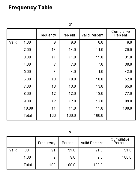
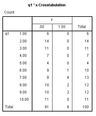
socst v1 v2 v3 v4 v5 36.00 . . . . . 61.00 37.00 38.00 39.00 40.00 41.00 46.00 62.00 63.00 64.00 65.00 66.00 36.00 47.00 48.00 49.00 50.00 51.00 51.00 37.00 38.00 39.00 40.00 41.00 46.00 52.00 53.00 54.00 55.00 56.00 42.00 47.00 48.00 49.00 50.00 51.00 46.00 43.00 44.00 45.00 46.00 47.00 51.00 47.00 48.00 49.00 50.00 51.00 36.00 52.00 53.00 54.00 55.00 56.00 Number of cases read: 10 Number of cases listed: 10* second example - looping down cases. set seed 95131257. input program. loop case_num=1 to 100. compute q1=trunc(uniform(10)+1). end case. end loop. end file. end input program. exe. compute x = 0. if q1=lag(Q1) x=1. list case_num q1 x /cases from 1 to 10.case_num q1 x 1.00 8.00 .00 2.00 10.00 .00 3.00 9.00 .00 4.00 2.00 .00 5.00 7.00 .00 6.00 7.00 1.00 7.00 3.00 .00 8.00 10.00 .00 9.00 4.00 .00 10.00 8.00 .00 Number of cases read: 10 Number of cases listed: 10frequencies var =q1 x.
crosstabs
/tables = q1 by x.


