Introduction
Panel data analysis, also known as cross-sectional time-series analysis, looks at a group of people, the ‘panel,’ on more than one occasion. Panel studies are essentially equivalent to longitudinal studies, although there may be many response variables observed at each time point.
These data are from a 1996 study (Gregoire, Kumar Everitt, Henderson and Studd) on the efficacy of estrogen patches in treating postnatal depression. Women were randomly assigned to either a placebo control group (group=0, n=27) or estrogen patch group (group=1, n=34). Prior to the first treatment all patients took the Edinburgh Postnatal Depression Scale (EPDS). EPDS data was collected monthly for six months once the treatment began. Higher scores on the EDPS are indicative of higher levels of depression. You can download the data file here.
get file = 'D:\depress-3.sav'.
Let the analyses begin
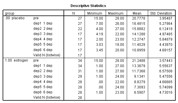
Note that the data are in the wide format, we will collect some information and perform two analyses while the data are in this format.
sort cases by group.
split file by group.
descriptives var = pre dep1 dep2 dep3 dep4 dep5 dep6.
split file off.
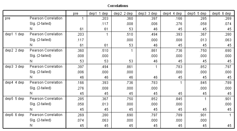
correlations var = pre dep1 dep2 dep3 dep4 dep5 dep6.
graph
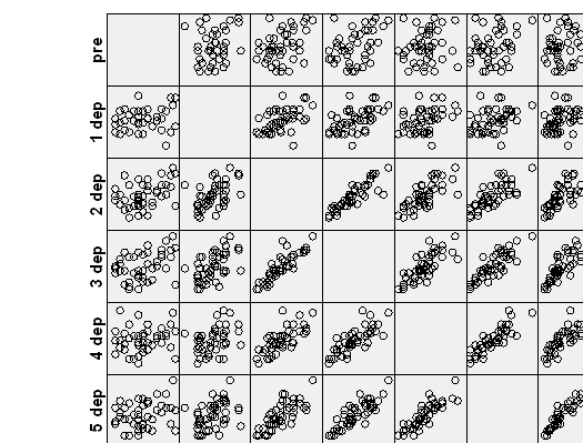
 /scatterplot(matrix) = pre dep1 dep2 dep3 dep4 dep5 dep6.
Let’s check to see if the groups differ on the pretest depression score.
t-test groups = group(0 1)
 /var = pre.
There isn’t much of a difference between groups on the pretest, so let’s continue on to the panel data analysis.
GEE with Continuous Response Variable
In order to use these data for our panel data analysis, the data must be reorganized into the long form using the varstocases command.
varstocases
 /make dep from dep1 dep2 dep3 dep4 dep5 dep6
 /index = visit.
Before we begin the panel data analyses, let’s look at some other analyses for comparison. We will begin with a repeated measures analysis of variance.
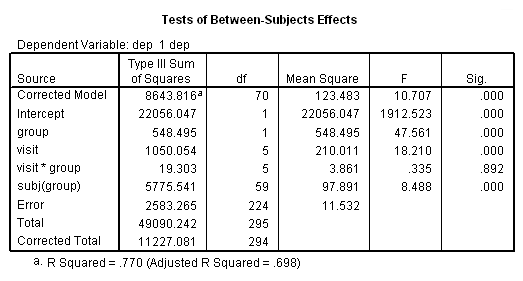
unianova dep by visit group subj
 /test =group vs subj(group)
 /design = group visit group*visit subj(group).
This analysis indicates that both group (F = 5.6, p = .021) and visit (F = 18.21, p = .000) are statistically significant, while the group*visit interaction is not (F = .335, p = .892). Some researchers are critical of this type of analysis because it is based on fixed-effects adjusted for the repeated factor. Also, this repeated measures analysis assumes compound symmetry in the covariance matrix (which seems to be a stretch in this case). However, we can do worse. Below we will try OLS regression.
regression
 /dependent = dep
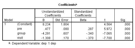
 /method = enter pre group visit.
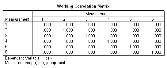
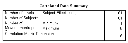
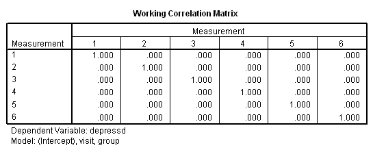
We are finally ready to try the panel data analysis using SPSS’s genlin command. This command allows us to specify various working covariance structures through the use of the corrtype option on the repeated subcommand. We will start with a covariance structure of independence. We don’t believe that this is the correct covariance structure, but it allows us to compare results with the OLS regression results above. The workingcorr option on the print subcommand will allow us to view the working correlation matrix. Note that this option is only available if the repeated subcommand is used. (The genlin command was introduced in SPSS version 15 and enhanced in version 16. If you are using an earlier version of SPSS, this command will not work.)
genlin dep with pre visit group
 /model pre group visit distribution = normal link = identity
 /repeated subject = subj
 /print modelinfo cps solution workingcorr.
The previous analyses yielded identical but probably incorrect results. The common thread among them is that they all assume that the observations within subjects are independent. This seems, on the face of it, to be highly unlikely. Scores on the depression scale are not likely to be independent from one visit to the next.
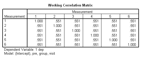
We can also try analyzing these data using compound symmetry for the correlational structure. Compound symmetry is obtained using exchangable for the corrtype option.
genlin dep with pre visit group
 /model pre visit group distribution = normal link = identity
 /repeated subject = subj corrtype = exchangeable
 /print modelinfo cps solution workingcorr.
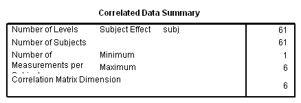
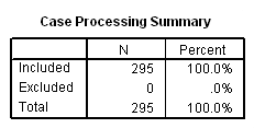
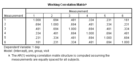
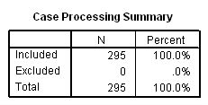
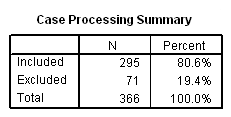
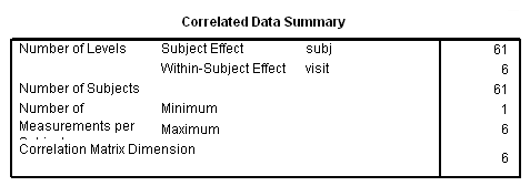
Note in particular the change in the standard errors between this analysis and the previous one. Now, let’s try a different correlation structure, auto regressive with lag one. This is the correlational structure that is most likely to be correct considering the repeated measures over time. I should note that, in some cases, SPSS and SAS handle models with an ar(1) structure differently than other packages, such as Stata. Stata does not use subjects that have only observation, since ar(1) doesn’t make much sense given one data point. SPSS and SAS use all of the available cases. You can see how many cases SPSS is using the Case Processing Summary table.
genlin dep with pre visit group
 /model pre group visit distribution = normal link = identity
 /repeated subject = subj corrtype = ar(1)
 /print modelinfo cps solution workingcorr.
This analysis probably more closely reflects the correlations among the depression scores over six visits that we observed in our descriptive analysis.
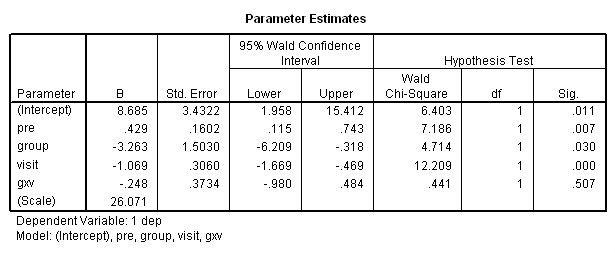
Now, let’s back up and reconsider the group by visit interaction. We will try a model with the interaction using the ar1 correlations. Note that we have omitted some of the output in order to save space.
compute gxv = group*visit.
exe.
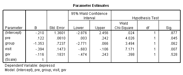
genlin dep with pre visit group gxv /model pre group visit gxv distribution = normal link = identity /repeated subject = subj corrtype = ar(1).
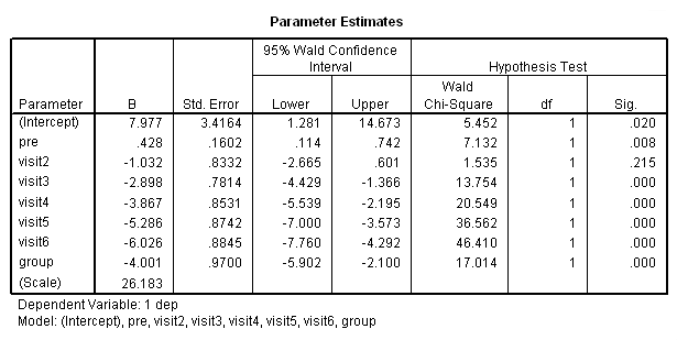
The group by visit interaction still is not significant, even though this may be a better approach for testing it. So far we have been treating visit as a continuous variable. Is it possible that our analysis might change if we were to treat visit as a categorical variable, in the way that the ANOVA did?
compute visit2 = 0.
if visit = 2 visit2 = 1.
compute visit3 = 0.
if visit = 3 visit3 = 1.
compute visit4 = 0.
if visit = 4 visit4 = 1.
compute visit5 = 0.
if visit = 5 visit5 = 1.
compute visit6 = 0.
if visit = 6 visit6 = 1.
exe.
genlin dep with pre visit2 visit3 visit4 visit5 visit6 group /model pre visit2 visit3 visit4 visit5 visit6 group distribution = normal link = identity /repeated subject = subj corrtype = ar(1).
In the final analysis, I think that I prefer the following model:
genlin dep with pre visit group
 /model pre group visit distribution = normal link = identity
 /repeated subject = subj corrtype = ar(1).
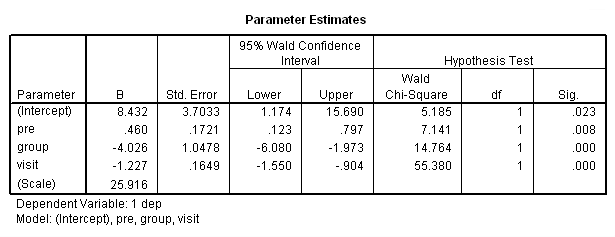
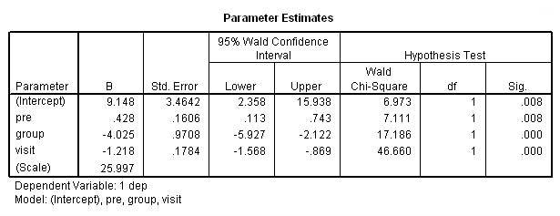
of all the analyses run so far. Those results looked as follows:
The final interpretation of these results indicate that there is a significant effect for the pretest, i.e., for every one point increase in the pretest score there is about a 0.4 increase in the depression score, when controlling for treatment and visit. There is also an effect for the estrogen patch when controlling for pretest depression and visit. Use of the estrogen patch reduces the depression score by 4 points. Finally, there is also a significant visit effect when controlling for pretest depression and group membership. The depression score decreases on the average by 1.2 points for each visit.
GEE with Binary Response Variable
The binary response variable in these examples was created from the data from the 1996 Gregoire, Kumar Everitt, Henderson and Studd study on the efficacy of estrogen patches in treating postnatal depression. Women were randomly assigned to either a placebo control group (group=0, n=27) or estrogen patch group (group=1, n=34). Prior to the first treatment all patients took the Edinburgh Postnatal Depression Scale (EPDS). EPDS data was collected monthly for six months once the treatment began. Depression scores greater than or equal to 11 were coded as 1. You can download the data file here.
get file = 'D:\depressed01.sav'.
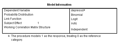
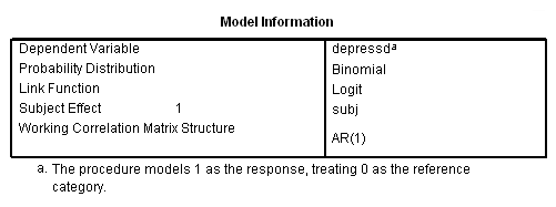
We will go through as series of analyses pretty much paralleling models that were run above using the continuous response variable. To get a binary logit type model we will set distribution to binomial and link to logit. We will start with the correlation structure independent follow by exchangeable (compound symmetry) and then unstructured.
genlin depressd (reference = first) with visit group
 /model visit group distribution = binomial link = logit
 /repeated subject = subj
 /print modelinfo cps solution workingcorr.
genlin depressd (reference = first) with visit group
 /model visit group distribution = binomial link = logit
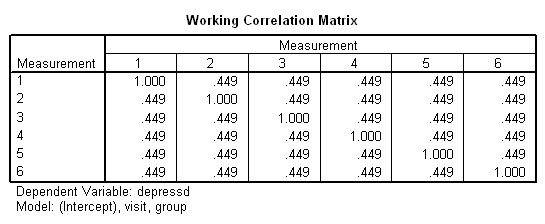
 /repeated subject = subj corrtype = exchangeable
 /print modelinfo cps solution workingcorr.
genlin depressd (reference = first) with visit group
 /model visit group distribution = binomial link = logit
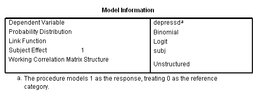
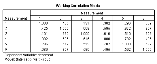
 /repeated subject = subj corrtype = unstructured
 /print modelinfo cps solution workingcorr.
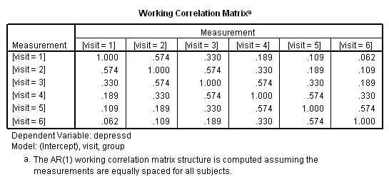
With these data, just as with the continuous response variable, it might be more reasonable to hypothesize that the correlation structure would be autoregressive.
genlin depressd (reference = first) with visit group
 /model visit group distribution = binomial link = logit
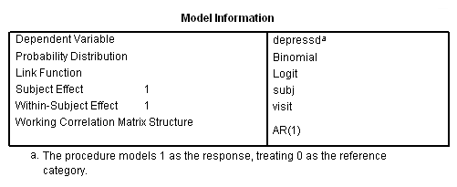
 /repeated subject = subj withinsubject=visit corrtype = ar(1) covb=model
 /print modelinfo cps solution workingcorr.
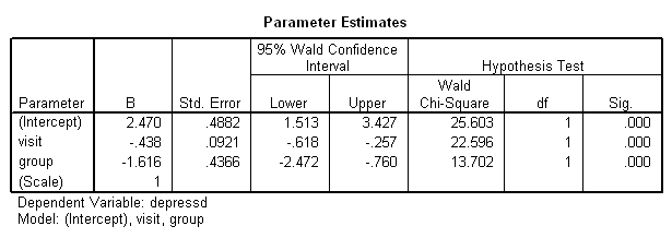
If we want, we can also obtain the results in the odds ratio metric using the exponentiated option on the print subcommand.
genlin depressd (reference = first) with visit group
 /model visit group distribution = binomial link = logit
 /repeated subject = subj corrtype = ar(1)
 /print solution (exponentiated) modelinfo.
Let’s add in the pretest (pre) and a group by visit interaction.
compute gxv = group*visit.

genlin depressd (reference = first) with pre group visit gxv
 /model pre group visit gxv distribution = binomial link = logit
 /repeated subject = subj corrtype = ar(1)
 /print solution modelinfo.
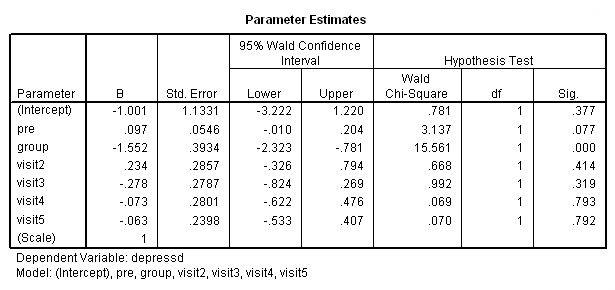
Clearly, there is no interaction but we’ll stick with the pretest for the moment. Next let’s try the categorical version of visit and the model that contains both the categorical and continuous version of visit.
compute visit2 = 0.
if visit = 2 visit2 = 1.
compute visit3 = 0.
if visit = 3 visit3 = 1.
compute visit4 = 0.
if visit = 4 visit4 = 1.
compute visit5 = 0.
if visit = 5 visit5 = 1.
compute visit6 = 0.
if visit = 6 visit6 = 1.
exe.

genlin depressd (reference = first) with pre group visit2 visit3 visit4 visit5
 /model pre group visit2 visit3 visit4 visit5 distribution = binomial link = logit
 /repeated subject = subj corrtype = ar(1)
 /print solution modelinfo.

