This learning module illustrates how to reshape data files in SPSS versions 11 and up. These examples take long data files and reshape them into wide form. Common examples of reshaping data are shown, but they do not exhaustively demonstrate the different kinds of data reshaping that you could encounter.
Example #1: One variable
Let’s use the https://stats.idre.ucla.edu/wp-content/uploads/2016/02/kidslw.sav file for our first example.
get file 'c:https://stats.idre.ucla.edu/wp-content/uploads/2016/02/kidslw.sav'.
list famid birth age.

    FAMID     BIRTH       AGE

     1.00      1.00      9.00
     1.00      2.00      6.00
     1.00      3.00      3.00
     2.00      1.00      8.00
     2.00      2.00      6.00
     2.00      3.00      2.00
     3.00      1.00      6.00
     3.00      2.00      4.00
     3.00      3.00      2.00

Number of cases read:  9    Number of cases listed:  9
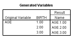
Let’s make the variable age in this file wide, making one record per family which would contain age1, age2 and age3, the ages of the kids in the family (age2 would be missing if there is only one kid, and age3 would be missing if there are only two kids). We will use the SPSS command casestovars to reshape the data from long to wide. On the /id subcommand, we list the name of the variable on which we want SPSS to "break" the data. Note that the data need to be sorted on the variable listed on the /id subcommand. We use the variable birth as the index variable on the /index subcommand. This is the variable that is controlling the naming of the variables in the new data set. Because birth has two decimal places, as seen in the output above, the new variables have .00 at the end of the names. If you do not want that, you can change the number of decimal places associated with the index variable. Using the point-and-click interface, you can do this in the "Variable View" window in the column called "Decimals", or if you would rather use syntax, you can use the formats command. We list on the /drop subcommand all of the other variables in the data set. Any variable that you do not list on the /drop subcommand will be reshaped.
casestovars
 /id=famid
 /index = birth
 /drop id kidname wt sex.
list.
FAMID AGE.1.00 AGE.2.00 AGE.3.00 1.00 9.00 6.00 3.00 2.00 8.00 6.00 2.00 3.00 6.00 4.00 2.00 Number of cases read: 3 Number of cases listed: 3
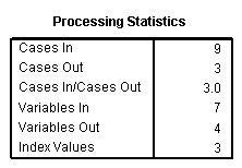
Also note that in the output, SPSS tells us which variable were used to create the new variables, how many cases were in the long data set (called "Cases In" in the Processing Statistics table), how many cases are in the wide data set (called "Cases Out"), and how many index values were created. You can use this information to ensure that the reshaping went as desired.
Example #2: Two variables
In the example above, we reshaped only one variable, age. In the example below, we reshape the variables age and wt. You can reshape as many variables as needed by not including them on the /drop subcommand.
get file 'c:https://stats.idre.ucla.edu/wp-content/uploads/2016/02/kidslw.sav'.
list famid birth age.

       ID     FAMID BIRTH     AGE

     1.00      1.00 1.00      9.00
     2.00      1.00 2.00      6.00
     3.00      1.00 3.00      3.00
     4.00      2.00 1.00      8.00
     5.00      2.00 2.00      6.00
     6.00      2.00 3.00      2.00
     7.00      3.00 1.00      6.00
     8.00      3.00 2.00      4.00
     9.00      3.00 3.00      2.00

Number of cases read:  9    Number of cases listed:  9
casestovars /id=famid /index=birth /drop id kidname sex. list famid age.1.00 age.2.00 age.3.00 wt.1.00 wt.2.00 wt.3.00.FAMID AGE.1.00 AGE.2.00 AGE.3.00 WT.1.00 WT.2.00 WT.3.00 1.00 9.00 6.00 3.00 60.00 40.00 20.00 2.00 8.00 6.00 2.00 80.00 50.00 20.00 3.00 6.00 4.00 2.00 60.00 40.00 20.00 Number of cases read: 3 Number of cases listed: 3
Example #3: Both numeric and character variables
The examples above showed how to reshape data using numeric variables, but sometimes you will need to reshape character (i.e., string) variables as well. In this example, we reshape two numeric variables, age and wt, and two string variables, sex and kidname.
Consider the kidslw data file shown below.
get file 'c:https://stats.idre.ucla.edu/wp-content/uploads/2016/02/kidslw.sav'.
list.

       ID     FAMID KIDNAME     BIRTH       AGE        WT SEX

     1.00      1.00 Beth         1.00      9.00     60.00 f
     2.00      1.00 Bob          2.00      6.00     40.00 m
     3.00      1.00 Barb         3.00      3.00     20.00 f
     4.00      2.00 Andy         1.00      8.00     80.00 m
     5.00      2.00 Al           2.00      6.00     50.00 m
     6.00      2.00 Ann          3.00      2.00     20.00 f
     7.00      3.00 Pete         1.00      6.00     60.00 m
     8.00      3.00 Pam          2.00      4.00     40.00 f
     9.00      3.00 Phil         3.00      2.00     20.00 m

Number of cases read:  9    Number of cases listed:  9

casestovars
 /id=famid
 /drop id birth.
list famid v1 v2 v3 age.1 age.2 age.3 wt.1 wt.2 wt.3 sex.1 sex.2 sex.3.
The variables are listed in the following order: LINE 1: FAMID V1 V2 V3 AGE.1.00 AGE.2.00 AGE.3.00 WT.1.00 LINE 2: WT.2.00 WT.3.00 SEX.1.00 SEX.2.00 SEX.3.00 FAMID: 1.00 Beth Bob Barb 9.00 6.00 3.00 60.00 WT.2.00: 40.00 20.00 f m f FAMID: 2.00 Andy Al Ann 8.00 6.00 2.00 80.00 WT.2.00: 50.00 20.00 m m f FAMID: 3.00 Pete Pam Phil 6.00 4.00 2.00 60.00 WT.2.00: 40.00 20.00 m f m Number of cases read: 3 Number of cases listed: 3
The warning message below is part of the SPSS output.
As you can see, SPSS has renamed some of the variables with names that are not very informative. We can use the /rename subcommand to rename the variables to meaningful names.
get file "c:https://stats.idre.ucla.edu/wp-content/uploads/2016/02/kidslw.sav".casestovars /id=famid /rename kidname=n /index=birth /drop id sex. list famid n.1.00 n.2.00 n.3.00 age.1.00 age.2.00 age.3.00 wt.1.00 wt.2.00 wt.3.00.The variables are listed in the following order: LINE 1: FAMID N.1.00 N.2.00 N.3.00 AGE.1.00 AGE.2.00 AGE.3.00 WT.1.00 LINE 2: WT.2.00 WT.3.00 FAMID: 1.00 Beth Bob Barb 9.00 6.00 3.00 60.00 WT.2.00: 40.00 20.00 FAMID: 2.00 Andy Al Ann 8.00 6.00 2.00 80.00 WT.2.00: 50.00 20.00 FAMID: 3.00 Pete Pam Phil 6.00 4.00 2.00 60.00 WT.2.00: 40.00 20.00 Number of cases read: 3 Number of cases listed: 3
Another change that we can make to the naming of variables is altering the separator that is used between the root name and the index. For example, in the above output, the root names are name, age and wt; the indexes are 1, 2 and 3. These values are separated by periods (.), but we can change that using the /separator subcommand, as shown below. Also, we will use the formats command to change the format of birth so that it no longer has decimals.
get file "c:https://stats.idre.ucla.edu/wp-content/uploads/2016/02/kidslw.sav".
formats birth (f1).

casestovars
 /id=famid
 /index=birth
 /rename kidname=name
 /separator = "_"
 /drop id sex.
list famid name_1 name_2 name_3 age_1 age_2 age_3 wt_1 wt_2 wt_3.
The variables are listed in the following order: LINE 1: FAMID NAME_1 NAME_2 NAME_3 AGE_1 AGE_2 AGE_3 WT_1 LINE 2: WT_2 WT_3 FAMID: 1.00 Beth Bob Barb 9.00 6.00 3.00 60.00 WT_2: 40.00 20.00 FAMID: 2.00 Andy Al Ann 8.00 6.00 2.00 80.00 WT_2: 50.00 20.00 FAMID: 3.00 Pete Pam Phil 6.00 4.00 2.00 60.00 WT_2: 40.00 20.00 Number of cases read: 3 Number of cases listed: 3
Example #4: Character suffixes
Variables with character suffixes are not a problem with the casestovars command. Nothing needs to be done differently when you have character suffixes, as illustrated below. Note that in this example, the data file is not sorted on the variable that we will use as the id variable; therefore, we need to sort the data before reshaping it. We will use the file https://stats.idre.ucla.edu/wp-content/uploads/2016/02/dadmoml.sav .
get file 'c:https://stats.idre.ucla.edu/wp-content/uploads/2016/02/dadmoml.sav'.
list.
ID FAMID NAME INC DADMOM 1.00 2.00 Art 22000.00 dad 2.00 1.00 Bill 30000.00 dad 3.00 3.00 Paul 25000.00 dad 4.00 1.00 Bess 15000.00 mom 5.00 3.00 Pat 50000.00 mom 6.00 2.00 Amy 18000.00 mom Number of cases read: 6 Number of cases listed: 6sort cases by famid. casestovars /id=famid /drop=id /index=dadmom. list.FAMID NAME.DAD NAME.MOM INC.DAD INC.MOM 1.00 Bill Bess 30000.00 15000.00 2.00 Art Amy 22000.00 18000.00 3.00 Paul Pat 25000.00 50000.00 Number of cases read: 3 Number of cases listed: 3
Example #5: No index variable
There may be times when your data are ordered but an index variable is not present. This is not a problem, as there is no need for an index variable, as long as the data set is properly sorted (i.e., by famid and birth) and there are no missing values.
get file 'c:kidslw.sav'.
list famid birth age.
FAMID BIRTH AGE 1.00 1.00 9.00 1.00 2.00 6.00 1.00 3.00 3.00 2.00 1.00 8.00 2.00 2.00 6.00 2.00 3.00 2.00 3.00 1.00 6.00 3.00 2.00 4.00 3.00 3.00 2.00 Number of cases read: 9 Number of cases listed: 9casestovars /id=famid /drop id kidname birth wt sex. list famid age.1 age.2 age.3.FAMID AGE.1 AGE.2 AGE.3 1.00 9.00 6.00 3.00 2.00 8.00 6.00 2.00 3.00 6.00 4.00 2.00 Number of cases read: 3 Number of cases listed: 3
Example #6: A more complex example
In the example below, we have three variables, a, b and outcome. We would like to make the variable outcome wide, creating three variables containing the values in outcome in the long data set. We would like all of the values associated with b = 1 to be in the first column of outcome, all of the values associated with b = 2 in the second column of outcome, and all of the values associated with b = 3 in the third column of outcome. However, we do not have the variable that we would like to use on the /id subcommand. We will create this variable, which we will call index, using the compute and if commands and the lag function. The resulting data set is shown below.
get file "c:reshape.sav".
compute index = 1.
if b = lag(b) index = lag(index)+1.
execute.
list.

       A        B  OUTCOME    INDEX

    1.00     1.00     1.00     1.00
    1.00     1.00     4.00     2.00
    1.00     1.00     3.00     3.00
    1.00     1.00     4.00     4.00
    2.00     1.00     4.00     5.00
    2.00     1.00    34.00     6.00
    2.00     1.00    56.00     7.00
    2.00     1.00    67.00     8.00
    3.00     1.00    45.00     9.00
    3.00     1.00    53.00    10.00
    3.00     1.00   456.00    11.00
    3.00     1.00    56.00    12.00
    1.00     2.00    67.00     1.00
    1.00     2.00     8.00     2.00
    1.00     2.00   454.00     3.00
    1.00     2.00     6.00     4.00
    2.00     2.00     7.00     5.00
    2.00     2.00    45.00     6.00
    2.00     2.00     4.00     7.00
    2.00     2.00     5.00     8.00
    3.00     2.00     4.00     9.00
    3.00     2.00     6.00    10.00
    3.00     2.00     7.00    11.00
    3.00     2.00     8.00    12.00
    1.00     3.00     9.00     1.00
    1.00     3.00   565.00     2.00
    1.00     3.00     5.00     3.00
    1.00     3.00     4.00     4.00
    2.00     3.00    46.00     5.00
    2.00     3.00   657.00     6.00
    2.00     3.00     8.00     7.00
    2.00     3.00    67.00     8.00
    3.00     3.00   454.00     9.00
    3.00     3.00  6768.00    10.00
    3.00     3.00    45.00    11.00
    3.00     3.00    78.00    12.00

Number of cases read:  36    Number of cases listed:  36
Before we can reshape the data, we need to sort them by the variable that we will use on the /id subcommand. Also, we will drop the variable b. If we do not drop b, we will get three variables, called b.1, b.2 and b.3, that will be constants, each with the value of its index.
sort cases by index.
casestovars
 /id = index
 /drop b.
list.
INDEX A V1 V2 V3 1.00 1.00 1.00 67.00 9.00 2.00 1.00 4.00 8.00 565.00 3.00 1.00 3.00 454.00 5.00 4.00 1.00 4.00 6.00 4.00 5.00 2.00 4.00 7.00 46.00 6.00 2.00 34.00 45.00 657.00 7.00 2.00 56.00 4.00 8.00 8.00 2.00 67.00 5.00 67.00 9.00 3.00 45.00 4.00 454.00 10.00 3.00 53.00 6.00 6768.00 11.00 3.00 456.00 7.00 45.00 12.00 3.00 56.00 8.00 78.00 Number of cases read: 12 Number of cases listed: 12


