This page shows examples of how to obtain descriptive statistics, with footnotes explaining the output. The data used in these examples were collected on 200 high schools students and are scores on various tests, including science, math, reading and social studies (socst). The variable female is a dichotomous variable coded 1 if the student was female and 0 if male.
In the syntax below, the get file command is used to load the data into SPSS. In quotes, you need to specify where the data file is located on your computer. Remember that you need to use the .sav extension and that you need to end the command (and all commands) with a period. There are several commands that you can use to get descriptive statistics for a continuous variable. We will show two: descriptives and examine. We have added some options to each of these commands, and we have deleted unnecessary subcommands to make the syntax as short and understandable as possible. You will find that the examine command always produces a lot of output. This can be very helpful if you know what you are looking for, but can be overwhelming if you are not used to it. If you need just a few numbers, you may want to use the descriptives command. Each as shown below.
We will use the hsb2.sav data file for our example.
get file "c:\data\hsb2.sav".

descriptives write
 /statistics = mean stddev variance min max semean kurtosis skewness.

descriptives write
 /statistics = mean stddev variance min max semean kurtosis skewness.

a. Valid N (listwise) – This is the number of non-missing values.
b. N – This is the number of valid observations for the variable. The total number of observations is the sum of N and the number of missing values.
c. Minimum – This is the minimum, or smallest, value of the variable.
d. Maximum – This is the maximum, or largest, value of the variable.
e. Mean – This is the arithmetic mean across the observations. It is the most widely used measure of central tendency. It is commonly called the average. The mean is sensitive to extremely large or small values.
f. Std. – Standard deviation is the square root of the variance. It measures the spread of a set of observations. The larger the standard deviation is, the more spread out the observations are.
g. Variance – The variance is a measure of variability. It is the sum of the squared distances of data value from the mean divided by the variance divisor. The Corrected SS is the sum of squared distances of data value from the mean. Therefore, the variance is the corrected SS divided by N-1. We don’t generally use variance as an index of spread because it is in squared units. Instead, we use standard deviation.
h. Skewness – Skewness measures the degree and direction of asymmetry. A symmetric distribution such as a normal distribution has a skewness of 0, and a distribution that is skewed to the left, e.g. when the mean is less than the median, has a negative skewness.
i. Kurtosis – Kurtosis is a measure of tail extremity reflecting either the presence of outliers in a distribution or a distribution’s propensity for producing outliers (Westfall,2014)
examine write
 /plot boxplot stemleaf histogram
 /percentiles(5,10,25,50,75,90,95,99).


writing score Stem-and-Leaf Plot
Frequency Stem & Leaf
     4.00        3 .  1111
     4.00        3 .  3333
     2.00        3 .  55
     5.00        3 .  66777
     6.00        3 .  899999
    13.00        4 .  0001111111111
     3.00        4 .  223
    13.00        4 .  4444444444445
    11.00        4 .  66666666677
    11.00        4 .  99999999999
     2.00        5 .  00
    16.00        5 .  2222222222222223
    20.00        5 .  44444444444444444555
    12.00        5 .  777777777777
    25.00        5 .  9999999999999999999999999
     8.00        6 .  00001111
    22.00        6 .  2222222222222222223333
    16.00        6 .  5555555555555555
     7.00        6 .  7777777
 Stem width:     10.00
 Each leaf:       1 case(s)
examine write
 /plot boxplot stemleaf histogram
 /percentiles(5,10,25,50,75,90,95,99).
Case processing summary

a. Valid – This refers to the non-missing cases. In this column, the N is given, which is the number of non-missing cases; and the Percent is given, which is the percent of non-missing cases.
b. Missing – This refers to the missing cases. In this column, the N is given, which is the number of missing cases; and the Percent is given, which is the percent of the missing cases.
c. Total – This refers to the total number cases, both non-missing and missing. In this column, the N is given, which is the total number of cases in the data set; and the Percent is given, which is the total percent of cases in the data set.
Descriptive statistics
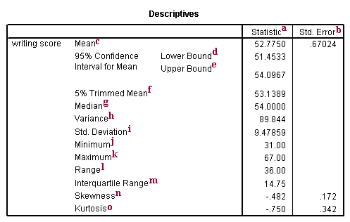
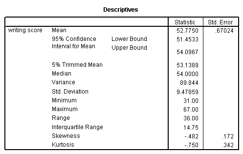
a. Statistic – These are the descriptive statistics.
b. Std. Error – These are the standard errors for the descriptive statistics. The standard error gives some idea about the variability possible in the statistic.
c. Mean – This is the arithmetic mean across the observations. It is the most widely used measure of central tendency. It is commonly called the average. The mean is sensitive to extremely large or small values.
d. 95% Confidence Interval for Mean Lower Bound – This is the lower (95%) confidence limit for the mean. If we repeatedly drew samples of 200 students’ writing test scores and calculated the mean for each sample, we would expect that 95% of them would fall between the lower and the upper 95% confidence limits. This gives you some idea about the variability of the estimate of the true population mean.
e. 95% Confidence Interval for Mean Upper Bound – This is the upper (95%) confidence limit for the mean.
f. 5% Trimmed Mean – This is the mean that would be obtained if the lower and upper 5% of values of the variable were deleted. If the value of the 5% trimmed mean is very different from the mean, this indicates that there are some outliers. However, you cannot assume that all outliers have been removed from the trimmed mean.
g. Median – This is the median. The median splits the distribution such that half of all values are above this value, and half are below.
h. Variance – The variance is a measure of variability. It is the sum of the squared distances of data value from the mean divided by the variance divisor. The Corrected SS is the sum of squared distances of data value from the mean. Therefore, the variance is the corrected SS divided by N-1. We don’t generally use variance as an index of spread because it is in squared units. Instead, we use standard deviation.
i. St. Deviation – Standard deviation is the square root of the variance. It measures the spread of a set of observations. The larger the standard deviation is, the more spread out the observations are.
j. Minimum – This is the minimum, or smallest, value of the variable.
k. Maximum – This is the maximum, or largest, value of the variable.
l. Range – The range is a measure of the spread of a variable. It is equal to the difference between the largest and the smallest observations. It is easy to compute and easy to understand. However, it is very insensitive to variability.
m. Interquartile Range – The interquartile range is the difference between the upper and the lower quartiles. It measures the spread of a data set. It is robust to extreme observations.
n. Skewness – Skewness measures the degree and direction of asymmetry. A symmetric distribution such as a normal distribution has a skewness of 0, and a distribution that is skewed to the left, e.g. when the mean is less than the median, has a negative skewness.
o. Kurtosis – Kurtosis is a measure of the heaviness of the tails of a distribution. In SAS, a normal distribution has kurtosis 0. Extremely nonnormal distributions may have high positive or negative kurtosis values, while nearly normal distributions will have kurtosis values close to 0. Kurtosis is positive if the tails are “heavier” than for a normal distribution and negative if the tails are “lighter” than for a normal distribution.
Percentiles

a. Weighted Average – These are the percentiles for the variable write. Some of the values are fractional, which is a result of how they are calculated. If there is not a value at exactly the 5th percentile, for example, the value is interpolated. There are several different ways of calculating these values, so SPSS clarifies what it is doing by indicating that it is using “Definition 1”.
b. Tukey’s Hinges – These are the first, second and third quartile. They are calculated the way that Tukey originally proposed when he came up with the idea of a boxplot. The values are not interpolated; rather, they are approximations that can be obtained with little calculation.
c. Percentiles – These columns given you the values of the variable at various percentiles. These tell you about the distribution of the variable. Percentiles are determined by ordering the values of the variable from lowest to highest, and then looking at whatever percent to see the value of the variable there. For example, in the column labeled 5, the value of the variable write is 35. Because this is a weighted average, SPSS is taking into account the fact that there are several values of 35, which is why the weighted average is 35.05.
d. 25 – This is the 25% percentile, also known as the first quartile.
e. 50 – This is the 50% percentile, also know as the median. It is a measure of central tendency. It is the middle number when the values are arranged in ascending (or descending) order. Sometimes, the median is a better measure of central tendency than the mean. It is less sensitive than the mean to extreme observations.
f. 75 – This is the 75% percentile, also know as the third quartile.
Histogram

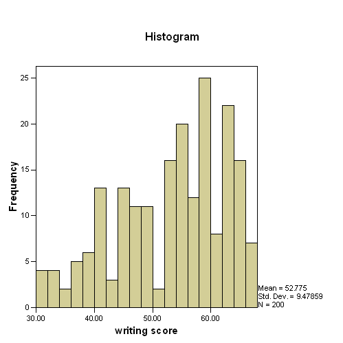
a. A histogram shows the frequency of values of a variable. The size of the bins is determined by default when you use the examine command to create a histogram, but you can use either the graph or ggraph command to create a histogram over which you can have much more control. In this histogram, each bin contains two values. For example, the first bin contains values 30 and 31, the second bin contains 32 and 33, and so on. The histogram is a graphical representation of the percentiles that were displayed above. As with percentiles, the purpose of the histogram is the give you an idea about the distribution of the variable.
Stem and leaf plot
writing score Stem-and-Leaf Plot
Frequencya Stemb& Leafc
     4.00        3 .  1111
     4.00        3 .  3333
     2.00        3 .  55
     5.00        3 .  66777
     6.00        3 .  899999
    13.00        4 .  0001111111111
     3.00        4 .  223
    13.00        4 .  4444444444445
    11.00        4 .  66666666677
    11.00        4 .  99999999999
     2.00        5 .  00
    16.00        5 .  2222222222222223
    20.00        5 .  44444444444444444555
    12.00        5 .  777777777777
    25.00        5 .  9999999999999999999999999
     8.00        6 .  00001111
    22.00        6 .  2222222222222222223333
    16.00        6 .  5555555555555555
     7.00        6 .  7777777
 Stem width:     10.00
 Each leaf:       1 case(s)
a. Frequency – This is the frequency of the leaves.
b. Stem – This is the stem. It is the number in the 10s place of the value of the variable. For example, in the first line, the stem is 3 and leaves are 1. The value of the variable is 31. The 3 is in the 10s place, so it is the stem.
c. Leaf – This is the leaf. It is the number in the 1s place of the value of the variable. The number of leaves tells you how many of these numbers is in the variable. For example, on the fifth line, there is one 8 and five 9s (hence, the frequency is six). This means that there is one value of 38 and five values of 39 in the variable write.
Boxplot
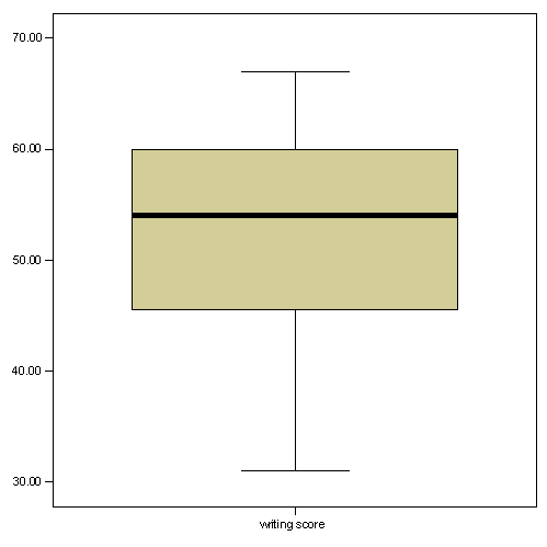
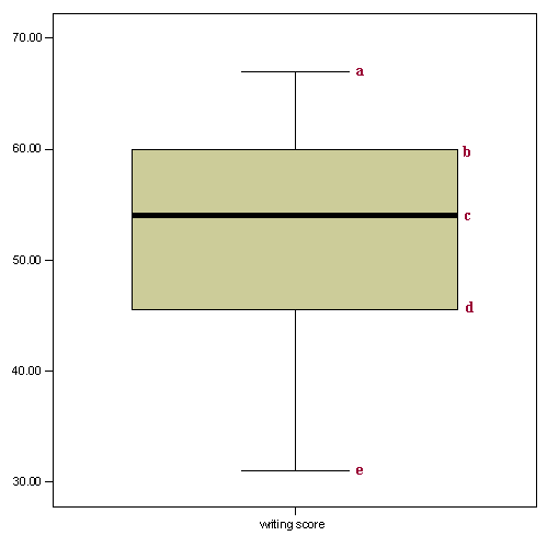
a. This is the maximmum score unless there are values more than 1.5 times the interquartile range above Q3, in which, it is the third quartile plus 1.5 times the interquartile range (the difference between the first and the third quartile).
b. This is the third quartile (Q3), also known as the 75th percentile.
c. This is the median (Q2), also known as the 50th percentile.
d. This is the first quartile (Q1), also known as the 25th percentile.
e. This is the minimum score unless there are values less than 1.5 times the interquartile range below Q1, in which case, it is the first quartile minus 1.5 times the interquartile range.
References:
- Westfall, P. Kurtosis as Peakedness, 1905 – 2014. R.I.P. Am Stat. 2014 ; 68(3): 191–195

