This page shows an example of a discriminant analysis in SPSS with footnotes explaining the output. The data used in this example are from a data file, https://stats.idre.ucla.edu/wp-content/uploads/2016/02/discrim.sav, with 244 observations on four variables. The variables include three continuous, numeric variables (outdoor, social and conservative) and one categorical variable (job) with three levels: 1) customer service, 2) mechanic and 3) dispatcher.
We are interested in the relationship between the three continuous variables and our categorical variable. Specifically, we would like to know how many dimensions we would need to express this relationship. Using this relationship, we can predict a classification based on the continuous variables or assess how well the continuous variables separate the categories in the classification. We will be discussing the degree to which the continuous variables can be used to discriminate between the groups. Some options for visualizing what occurs in discriminant analysis can be found in the Discriminant Analysis Data Analysis Example.
To start, we can examine the overall means of the continuous variables.
get file='C:\temp\discrim.sav'.
descriptives
 variables=outdoor social conservative
 /statistics=mean stddev min max .

We are interested in how job relates to outdoor, social and conservative. Let’s look at summary statistics of these three continuous variables for each job category.
means
  tables=outdoor social conservative by job
  /cells mean count stddev  .


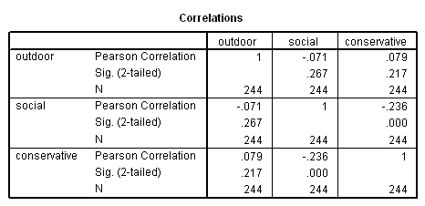
From this output, we can see that some of the means of outdoor, social and conservative differ noticeably from group to group in job. These differences will hopefully allow us to use these predictors to distinguish observations in one job group from observations in another job group. Next, we can look at the correlations between these three predictors. These correlations will give us some indication of how much unique information each predictor will contribute to the analysis. If two predictor variables are very highly correlated, then they will be contributing shared information to the analysis. Uncorrelated variables are likely preferable in this respect. We will also look at the frequency of each job group.
correlations
 variables=outdoor social conservative .
frequencies
 variables=job .


The discriminant command in SPSS performs canonical linear discriminant analysis which is the classical form of discriminant analysis. In this example, we specify in the groups subcommand that we are interested in the variable job, and we list in parenthesis the minimum and maximum values seen in job. We next list the discriminating variables, or predictors, in the variables subcommand. In this example, we have selected three predictors: outdoor, social and conservative. We will be interested in comparing the actual groupings in job to the predicted groupings generated by the discriminant analysis. For this, we use the statistics subcommand. This will provide us with classification statistics in our output.
discriminant
/groups=job(1 3)
/variables=outdoor social conservative
/statistics=table.
Data Summary
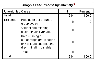
a. Analysis Case Processing Summary – This table summarizes the analysis dataset in terms of valid and excluded cases. The reasons why SPSS might exclude an observation from the analysis are listed here, and the number (“N”) and percent of cases falling into each category (valid or one of the exclusions) are presented. In this example, all of the observations in the dataset are valid.
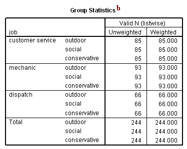
b. Group Statistics – This table presents the distribution of observations into the three groups within job. We can see the number of observations falling into each of the three groups. In this example, we are using the default weight of 1 for each observation in the dataset, so the weighted number of observations in each group is equal to the unweighted number of observations in each group.
Eigenvalues and Multivariate Tests
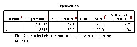

c. Function – This indicates the first or second canonical linear discriminant function. The number of functions is equal to the number of discriminating variables, if there are more groups than variables, or 1 less than the number of levels in the group variable. In this example, job has three levels and three discriminating variables were used, so two functions are calculated. Each function acts as projections of the data onto a dimension that best separates or discriminates between the groups.
d. Eigenvalue – These are the eigenvalues of the matrix product of the inverse of the within-group sums-of-squares and cross-product matrix and the between-groups sums-of-squares and cross-product matrix. These eigenvalues are related to the canonical correlations and describe how much discriminating ability a function possesses. The magnitudes of the eigenvalues are indicative of the functions’ discriminating abilities. See superscript e for underlying calculations.
e. % of Variance – This is the proportion of discriminating ability of the three continuous variables found in a given function. This proportion is calculated as the proportion of the function’s eigenvalue to the sum of all the eigenvalues. In this analysis, the first function accounts for 77% of the discriminating ability of the discriminating variables and the second function accounts for 23%. We can verify this by noting that the sum of the eigenvalues is 1.081+.321 = 1.402. Then (1.081/1.402) = 0.771 and (0.321/1.402) = 0.229.
f. Cumulative % – This is the cumulative proportion of discriminating ability . For any analysis, the proportions of discriminating ability will sum to one. Thus, the last entry in the cumulative column will also be one.
g. Canonical Correlation – These are the canonical correlations of our predictor variables (outdoor, social and conservative) and the groupings in job. If we consider our discriminating variables to be one set of variables and the set of dummies generated from our grouping variable to be another set of variables, we can perform a canonical correlation analysis on these two sets. From this analysis, we would arrive at these canonical correlations.
h. Test of Function(s) – These are the functions included in a given test with the null hypothesis that the canonical correlations associated with the functions are all equal to zero. In this example, we have two functions. Thus, the first test presented in this table tests both canonical correlations (“1 through 2”) and the second test presented tests the second canonical correlation alone.
i. Wilks’ Lambda – Wilks’ Lambda is one of the multivariate statistic calculated by SPSS. It is the product of the values of (1-canonical correlation2). In this example, our canonical correlations are 0.721 and 0.493, so the Wilks’ Lambda testing both canonical correlations is (1- 0.7212)*(1-0.4932) = 0.364, and the Wilks’ Lambda testing the second canonical correlation is (1-0.4932) = 0.757.
j. Chi-square – This is the Chi-square statistic testing that the canonical correlation of the given function is equal to zero. In other words, the null hypothesis is that the function, and all functions that follow, have no discriminating ability. This hypothesis is tested using this Chi-square statistic.
k. df – This is the effect degrees of freedom for the given function. It is based on the number of groups present in the categorical variable and the number of continuous discriminant variables. The Chi-square statistic is compared to a Chi-square distribution with the degrees of freedom stated here.
l. Sig. – This is the p-value associated with the Chi-square statistic of a given test. The null hypothesis that a given function’s canonical correlation and all smaller canonical correlations are equal to zero is evaluated with regard to this p-value. For a given alpha level, such as 0.05, if the p-value is less than alpha, the null hypothesis is rejected. If not, then we fail to reject the null hypothesis.
Discriminant Function Output
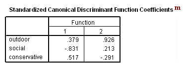
m. Standardized Canonical Discriminant Function Coefficients – These coefficients can be used to calculate the discriminant score for a given case. The score is calculated in the same manner as a predicted value from a linear regression, using the standardized coefficients and the standardized variables. For example, let zoutdoor, zsocial and zconservative be the variables created by standardizing our discriminating variables. Then, for each case, the function scores would be calculated using the following equations:
Score1 = 0.379*zoutdoor – 0.831*zsocial + 0.517*zconservative
Score2 = 0.926*zoutdoor + 0.213*zsocial – 0.291*zconservative
The distribution of the scores from each function is standardized to have a mean of zero and standard deviation of one. The magnitudes of these coefficients indicate how strongly the discriminating variables effect the score. For example, we can see that the standardized coefficient for zsocial in the first function is greater in magnitude than the coefficients for the other two variables. Thus, social will have the greatest impact of the three on the first discriminant score.
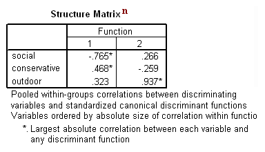
n. Structure Matrix – This is the canonical structure, also known as canonical loading or discriminant loading, of the discriminant functions. It represents the correlations between the observed variables (the three continuous discriminating variables) and the dimensions created with the unobserved discriminant functions (dimensions).
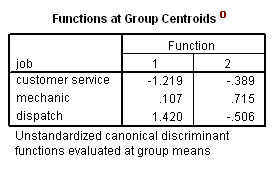
o. Functions at Group Centroids – These are the means of the discriminant function scores by group for each function calculated. If we calculated the scores of the first function for each case in our dataset, and then looked at the means of the scores by group, we would find that the customer service group has a mean of -1.219, the mechanic group has a mean of 0.107, and the dispatch group has a mean of 1.420. We know that the function scores have a mean of zero, and we can check this by looking at the sum of the group means multiplied by the number of cases in each group: (85*-1.219)+(93*.107)+(66*1.420) = 0.
Predicted Classifications
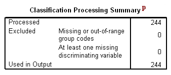
p. Classification Processing Summary – This is similar to the Analysis Case Processing Summary (see superscript a), but in this table, “Processed” cases are those that were successfully classified based on the analysis. The reasons why an observation may not have been processed are listed here. We can see that in this example, all of the observations in the dataset were successfully classified.
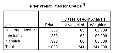
q. Prior Probabilities for Groups – This is the distribution of observations into the job groups used as a starting point in the analysis. The default prior distribution is an equal allocation into the groups, as seen in this example. SPSS allows users to specify different priors with the priors subcommand.
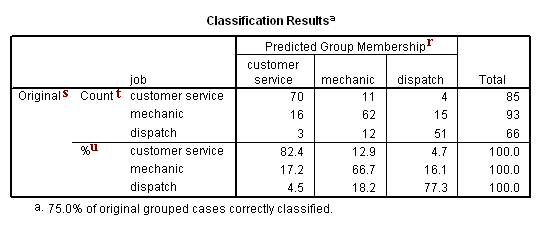
r. Predicted Group Membership – These are the predicted frequencies of groups from the analysis. The numbers going down each column indicate how many were correctly and incorrectly classified. For example, of the 85 cases that were predicted to be in the customer service group, 70 were correctly predicted, and 19 were incorrectly predicted (16 cases were in the mechanic group and three cases were in the dispatch group).
s. Original – These are the frequencies of groups found in the data. We can see from the row totals that 85 cases fall into the customer service group, 93 fall into the mechanic group, and 66 fall into the dispatch group. These match the results we saw earlier in the output for the frequencies command. Across each row, we see how many of the cases in the group are classified by our analysis into each of the different groups. For example, of the 85 cases that are in the customer service group, 70 were predicted correctly and 15 were predicted incorrectly (11 were predicted to be in the mechanic group and four were predicted to be in the dispatch group).
t. Count – This portion of the table presents the number of observations falling into the given intersection of original and predicted group membership. For example, we can see in this portion of the table that the number of observations originally in the customer service group, but predicted to fall into the mechanic group is 11. The row totals of these counts are presented, but column totals are not.
u. % – This portion of the table presents the percent of observations originally in a given group (listed in the rows) predicted to be in a given group (listed in the columns). For example, we can see that the percent of observations in the mechanic group that were predicted to be in the dispatch group is 16.1%. This is NOT the same as the percent of observations predicted to be in the dispatch group that were in the mechanic group. The latter is not presented in this table.
Appendix
The following code can be used to calculate the scores manually:
DESCRIPTIVES VARIABLES=outdoor social conservative
 /SAVE
 /STATISTICS=MEAN STDDEV MIN MAX.

COMPUTE Score1 = 0.379*Zoutdoor - 0.831*Zsocial + 0.517*Zconservative.
COMPUTE Score2 = 0.926*Zoutdoor - 0.213*Zsocial + 0.291*Zconservative.
Let’s take a look at the first two observations of the newly created scores:
LIST VARIABLES=Zoutdoor Zsocial Zconservative Score1 Score2
 /CASES=FROM 1 TO 2.

   Zoutdoor     Zsocial Zconservative   Score1   Score2

   -1.16517      .24160     -1.49999     -1.42    -1.57
    -.33871     -.67094     -1.23167      -.21     -.53


Number of cases read:  2    Number of cases listed:  2
Verify that the mean of the scores is zero and the standard deviation is roughly 1.
DESCRIPTIVES VARIABLES=Score1 Score2
 /STATISTICS=MEAN STDDEV MIN MAX.
| N | Minimum | Maximum | Mean | Std. Deviation | |
| Score1 | 244 | -3.20 | 3.31 | .0000 | 1.17481 |
| Score2 | 244 | -3.52 | 2.55 | .0000 | 1.04292 |
| Valid N (listwise) | 244 | ||||
