This page shows an example of logistic regression with footnotes explaining the output. These data were collected on 200 high schools students and are scores on various tests, including science, math, reading and social studies (socst). The variable female is a dichotomous variable coded 1 if the student was female and 0 if male.
In the syntax below, the get file command is used to load the hsb2 data into SPSS. In quotes, you need to specify where the data file is located on your computer. Remember that you need to use the .sav extension and that you need to end the command with a period. By default, SPSS does a listwise deletion of missing values. This means that only cases with non-missing values for the dependent as well as all independent variables will be used in the analysis.
Because we do not have a suitable dichotomous variable to use as our dependent variable, we will create one (which we will call honcomp, for honors composition) based on the continuous variable write. We do not advocate making dichotomous variables out of continuous variables; rather, we do this here only for purposes of this illustration.
Use the keyword with after the dependent variable to indicate all of the variables (both continuous and categorical) that you want included in the model. If you have a categorical variable with more than two levels, for example, a three-level ses variable (low, medium and high), you can use the categorical subcommand to tell SPSS to create the dummy variables necessary to include the variable in the logistic regression, as shown below. You can use the keyword by to create interaction terms. For example, the command logistic regression honcomp with read female read by female. will create a model with the main effects of read and female, as well as the interaction of read by female.
We will start by showing the SPSS commands to open the data file, creating the dichotomous dependent variable, and then running the logistic regression. We will show the entire output, and then break up the output with explanation.
get file "c:\data\hsb2.sav".

compute honcomp = (write ge 60).
exe.

logistic regression honcomp with read science ses
/categorical ses.
Logistic Regression

Block 0: Beginning Block

Block 1: Method = Enter
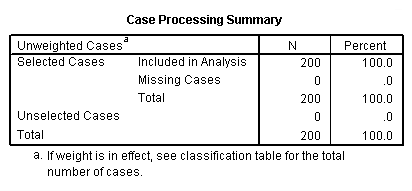
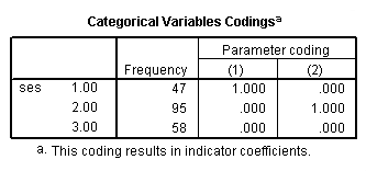
This part of the output tells you about the cases that were included and excluded from the analysis, the coding of the dependent variable, and coding of any categorical variables listed on the categorical subcommand. (Note: You will not get the third table (“Categorical Variable Codings”) if you do not specify the categorical subcommand.)
Logistic Regression
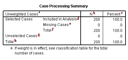
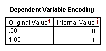
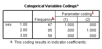
b. N – This is the number of cases in each category (e.g., included in the analysis, missing, total).
c. Percent – This is the percent of cases in each category (e.g., included in the analysis, missing, total).
d. Included in Analysis – This row gives the number and percent of cases that were included in the analysis. Because we have no missing data in our example data set, this also corresponds to the total number of cases.
e. Missing Cases – This row give the number and percent of missing cases. By default, SPSS logistic regression does a listwise deletion of missing data. This means that if there is missing value for any variable in the model, the entire case will be excluded from the analysis.
f. Total – This is the sum of the cases that were included in the analysis and the missing cases. In our example, 200 + 0 = 200.
Unselected Cases – If the select subcommand is used and a logical condition is specified with a categorical variable in the dataset, then the number of unselected cases would be listed here. Using the select subcommand is different from using the filter command. When the select subcommand is used, diagnostic and residual values are computed for all cases in the data. If the filter command is used to select cases to be used in the analysis, residual and diagnostic values are not computed for unselected cases.
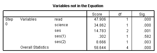
This part of the output describes a “null model”, which is model with no predictors and just the intercept. This is why you will see all of the variables that you put into the model in the table titled “Variables not in the Equation”.
Block 0: Beginning Block
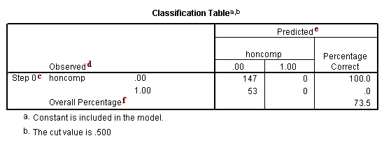

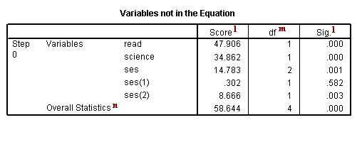
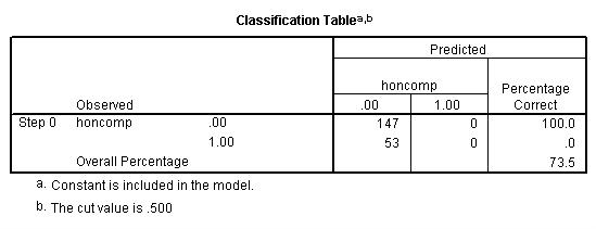
c. Step 0 – SPSS allows you to have different steps in your logistic regression model. The difference between the steps is the predictors that are included. This is similar to blocking variables into groups and then entering them into the equation one group at a time. By default, SPSS logistic regression is run in two steps. The first step, called Step 0, includes no predictors and just the intercept. Often, this model is not interesting to researchers.
d. Observed – This indicates the number of 0’s and 1’s that are observed in the dependent variable.
e. Predicted – In this null model, SPSS has predicted that all cases are 0 on the dependent variable.
f. Overall Percentage – This gives the percent of cases for which the dependent variables was correctly predicted given the model. In this part of the output, this is the null model. 73.5 = 147/200.
g. B – This is the coefficient for the constant (also called the “intercept”) in the null model.
h. S.E. – This is the standard error around the coefficient for the constant.
i. Wald and Sig. – This is the Wald chi-square test that tests the null hypothesis that the constant equals 0. This hypothesis is rejected because the p-value (listed in the column called “Sig.”) is smaller than the critical p-value of .05 (or .01). Hence, we conclude that the constant is not 0. Usually, this finding is not of interest to researchers.
j. df – This is the degrees of freedom for the Wald chi-square test. There is only one degree of freedom because there is only one predictor in the model, namely the constant.
k. Exp(B) – This is the exponentiation of the B coefficient, which is an odds ratio. This value is given by default because odds ratios can be easier to interpret than the coefficient, which is in log-odds units. This is the odds: 53/147 = .361.
l. Score and Sig. – This is a Score test that is used to predict whether or not an independent variable would be significant in the model. Looking at the p-values (located in the column labeled “Sig.”), we can see that each of the predictors would be statistically significant except the first dummy for ses.
m. df – This column lists the degrees of freedom for each variable. Each variable to be entered into the model, e.g., read, science, ses(1) and ses(2), has one degree of freedom, which leads to the total of four shown at the bottom of the column. The variable ses is listed here only to show that if the dummy variables that represent ses were tested simultaneously, the variable ses would be statistically significant.
n. Overall Statistics – This shows the result of including all of the predictors into the model.
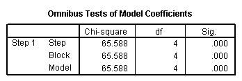
The section contains what is frequently the most interesting part of the output: the overall test of the model (in the “Omnibus Tests of Model Coefficients” table) and the coefficients and odds ratios (in the “Variables in the Equation” table).
Block 1: Method = Enter

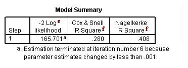

b. Step 1 – This is the first step (or model) with predictors in it. In this case, it is the full model that we specified in the logistic regression command. You can have more steps if you do stepwise or use blocking of variables.
c. Chi-square and Sig. – This is the chi-square statistic and its significance level. In this example, the statistics for the Step, Model and Block are the same because we have not used stepwise logistic regression or blocking. The value given in the Sig. column is the probability of obtaining the chi-square statistic given that the null hypothesis is true. In other words, this is the probability of obtaining this chi-square statistic (65.588) if there is in fact no effect of the independent variables, taken together, on the dependent variable. This is, of course, the p-value, which is compared to a critical value, perhaps .05 or .01 to determine if the overall model is statistically significant. In this case, the model is statistically significant because the p-value is less than .000.
d. df – This is the number of degrees of freedom for the model. There is one degree of freedom for each predictor in the model. In this example, we have four predictors: read, write and two dummies for ses (because there are three levels of ses).
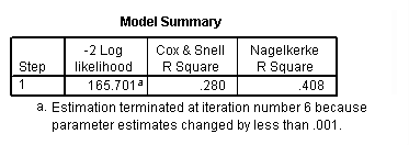
e. -2 Log likelihood – This is the -2 log likelihood for the final model. By itself, this number is not very informative. However, it can be used to compare nested (reduced) models.
f. Cox & Snell R Square and Nagelkerke R Square – These are pseudo R-squares. Logistic regression does not have an equivalent to the R-squared that is found in OLS regression; however, many people have tried to come up with one. There are a wide variety of pseudo-R-square statistics (these are only two of them). Because this statistic does not mean what R-squared means in OLS regression (the proportion of variance explained by the predictors), we suggest interpreting this statistic with great caution.
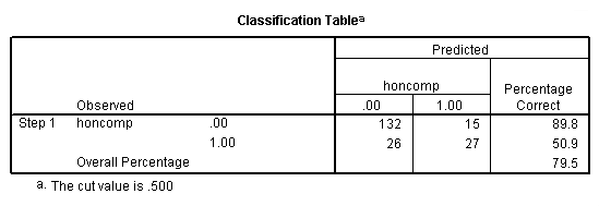
g. Observed – This indicates the number of 0’s and 1’s that are observed in the dependent variable.
h. Predicted – These are the predicted values of the dependent variable based on the full logistic regression model. This table shows how many cases are correctly predicted (132 cases are observed to be 0 and are correctly predicted to be 0; 27 cases are observed to be 1 and are correctly predicted to be 1), and how many cases are not correctly predicted (15 cases are observed to be 0 but are predicted to be 1; 26 cases are observed to be 1 but are predicted to be 0).
i. Overall Percentage – This gives the overall percent of cases that are correctly predicted by the model (in this case, the full model that we specified). As you can see, this percentage has increased from 73.5 for the null model to 79.5 for the full model.
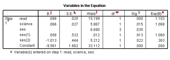
j. B – These are the values for the logistic regression equation for predicting the dependent variable from the independent variable. They are in log-odds units. Similar to OLS regression, the prediction equation is
log(p/1-p) = b0 + b1*x1 + b2*x2 + b3*x3 + b3*x3+b4*x4
where p is the probability of being in honors composition. Expressed in terms of the variables used in this example, the logistic regression equation is
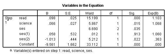
log(p/1-p) = –9.561 + 0.098*read + 0.066*science + 0.058*ses(1) – 1.013*ses(2)
These estimates tell you about the relationship between the independent variables and the dependent variable, where the dependent variable is on the logit scale. These estimates tell the amount of increase (or decrease, if the sign of the coefficient is negative) in the predicted log odds of honcomp = 1 that would be predicted by a 1 unit increase (or decrease) in the predictor, holding all other predictors constant. Note: For the independent variables which are not significant, the coefficients are not significantly different from 0, which should be taken into account when interpreting the coefficients. (See the columns labeled Wald and Sig. regarding testing whether the coefficients are statistically significant). Because these coefficients are in log-odds units, they are often difficult to interpret, so they are often converted into odds ratios. You can do this by hand by exponentiating the coefficient, or by looking at the right-most column in the Variables in the Equation table labeled “Exp(B)”. read – For every one-unit increase in reading score (so, for every additional point on the reading test), we expect a 0.098 increase in the log-odds of honcomp, holding all other independent variables constant. science – For every one-unit increase in science score, we expect a 0.066 increase in the log-odds of honcomp, holding all other independent variables constant. ses – This tells you if the overall variable ses is statistically significant. There is no coefficient listed, because ses is not a variable in the model. Rather, dummy variables which code for ses are in the equation, and those have coefficients. However, as you can see in this example, the coefficient for one of the dummies is statistically significant while the other one is not. The statistic given on this row tells you if the dummies that represent ses, taken together, are statistically significant. Because there are two dummies, this test has two degrees of freedom. This is equivalent to using the test statement in SAS or the test command is Stata. ses(1) – The reference group is level 3 (see the Categorical Variables Codings table above), so this coefficient represents the difference between level 1 of ses and level 3. Note: The number in the parentheses only indicate the number of the dummy variable; it does not tell you anything about which levels of the categorical variable are being compared. For example, if you changed the reference group from level 3 to level 1, the labeling of the dummy variables in the output would not change. ses(2) – The reference group is level 3 (see the Categorical Variables Codings table above), so this coefficient represents the difference between level 2 of ses and level 3. Note: The number in the parentheses only indicate the number of the dummy variable; it does not tell you anything about which levels of the categorical variable are being compared. For example, if you changed the reference group from level 3 to level 1, the labeling of the dummy variables in the output would not change. constant – This is the expected value of the log-odds of honcomp when all of the predictor variables equal zero. In most cases, this is not interesting. Also, oftentimes zero is not a realistic value for a variable to take.
k. S.E. – These are the standard errors associated with the coefficients. The standard error is used for testing whether the parameter is significantly different from 0; by dividing the parameter estimate by the standard error you obtain a t-value. The standard errors can also be used to form a confidence interval for the parameter.
l. Wald and Sig. – These columns provide the Wald chi-square value and 2-tailed p-value used in testing the null hypothesis that the coefficient (parameter) is 0. If you use a 2-tailed test, then you would compare each p-value to your preselected value of alpha. Coefficients having p-values less than alpha are statistically significant. For example, if you chose alpha to be 0.05, coefficients having a p-value of 0.05 or less would be statistically significant (i.e., you can reject the null hypothesis and say that the coefficient is significantly different from 0). If you use a 1-tailed test (i.e., you predict that the parameter will go in a particular direction), then you can divide the p-value by 2 before comparing it to your preselected alpha level. For the variable read, the p-value is .000, so the null hypothesis that the coefficient equals 0 would be rejected. For the variable science, the p-value is .015, so the null hypothesis that the coefficient equals 0 would be rejected. For the variable ses, the p-value is .035, so the null hypothesis that the coefficient equals 0 would be rejected. Because the test of the overall variable is statistically significant, you can look at the one degree of freedom tests for the dummies ses(1) and ses(2). The dummy ses(1) is not statistically significantly different from the dummy ses(3) (which is the omitted, or reference, category), but the dummy ses(2) is statistically significantly different from the dummy ses(3) with a p-value of .022.
m. df – This column lists the degrees of freedom for each of the tests of the coefficients.
n. Exp(B) – These are the odds ratios for the predictors. They are the exponentiation of the coefficients. There is no odds ratio for the variable ses because ses (as a variable with 2 degrees of freedom) was not entered into the logistic regression equation.
Odds Ratios
In this next example, we will illustrate the interpretation of odds ratios. In this example, we will simplify our model so that we have only one predictor, the binary variable female. Before we run the logistic regression, we will use the crosstabs command to obtain a crosstab of the two variables.
crosstabs female by honcomp.
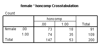
If we divide the number of males who are in honors composition, 18, by the number of males who are not in honors composition, 73, we get the odds of being in honors composition for males, 18/73 = .246. If we do the same thing for females, we get 35/74 = .472. To get the odds ratio, which is the ratio of the two odds that we have just calculated, we get .472/.246 = 1.918. As we can see in the output below, this is exactly the odds ratio we obtain from the logistic regression. The thing to remember here is that you want the group coded as 1 over the group coded as 0, so honcomp=1/honcomp=0 for both males and females, and then the odds for females/odds for males, because the females are coded as 1.
You can get the odds ratio from the crosstabs command by using the /statistics risk subcommand, as shown below.
crosstabs female by honcomp
 /statistics risk.
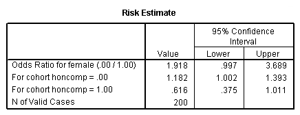
As you can see in the output below, we get the same odds ratio when we run the logistic regression. (NOTE: Although it is equivalent to the odds ratio estimated from the logistic regression, the odds ratio in the “Risk Estimate” table is calculated as the ratio of the odds of honcomp=0 for males over the odds of honcomp=0 for females, which explains the confusing row heading “Odds Ratio for female (.00/1.00)”). If we calculated a 95% confidence interval, we would not want this to include the value of 1. When we were considering the coefficients, we did not want the confidence interval to include 0. If we exponentiate 0, we get 1 (exp(0) = 1). Hence, this is two ways of saying the same thing. As you can see, the 95% confidence interval includes 1; hence, the odds ratio is not statistically significant. Because the lower bound of the 95% confidence interval is so close to 1, the p-value is very close to .05. We can use the /print = ic(95) subcommand to get the 95% confidence intervals included in our output.
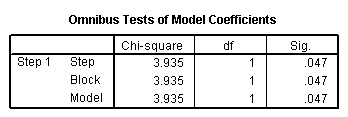
There are a few other things to note about the output below. The first is that although we have only one predictor variable, the test for the odds ratio does not match with the overall test of the model. This is because the test of the coefficient is a Wald chi-square test, while the test of the overall model is a likelihood ratio chi-square test. While these two types of chi-square tests are asymptotically equivalent, in small samples they can differ, as they do here. Also, we have the unfortunate situation in which the results of the two tests give different conclusions. This does not happen very often. In a situation like this, it is difficult to know what to conclude. One might consider the power, or one might decide if an odds ratio of this magnitude is important from a clinical or practical standpoint.
logistic regression honcomp with female
 /print = ci(95).

For more information on interpreting odds ratios, please see How do I interpret odds ratios in logistic regression? . Although this FAQ uses Stata for purposes of illustration, the concepts and explanations are useful.
