This page shows an example of a multinomial logistic regression analysis with footnotes explaining the output. The data were collected on 200 high school students and are scores on various tests, including a video game and a puzzle. The outcome measure in this analysis is the student’s favorite flavor of ice cream – vanilla, chocolate or strawberry- from which we are going to see what relationships exists with video game scores (video), puzzle scores (puzzle) and gender (female). The data set can be downloaded here.
get file = 'D:\data\mlogit.sav'.
Before running the regression, obtaining a frequency of the ice cream flavors in the data can inform the selection of a reference group. By default, SPSS uses the highest-numbered category as the reference category.
frequencies
/variables = ice_cream.

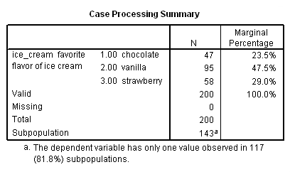
Vanilla is the most frequently preferred ice cream flavor and will be the reference group in this example. In the data, vanilla is represented by the number 2 (chocolate is 1, strawberry is 3). We will use the nomreg command to run the multinomial logistic regression.
The predictor variable female is coded 0 = male and 1 = female. In the analysis below, we treat the variable female as a continuous (i.e., a 1 degree of freedom) predictor variable by including it after the SPSS keyword with. If the predictor variable female was listed after the SPSS keyword by, SPSS would use 1 (females) as the reference group. Binary predictors can be listed after either the SPSS keyword with or by, depending on the preference of the analyst. For our example, we want males to be the reference group, so female is listed after with.
nomreg ice_cream (base = 2) with video puzzle female
/print = paramter summary cps mfi.
In the above command, base = 2 indicates which level of the outcome variable should be treated as the reference level. By default, SPSS sorts the groups and chooses the highest-numbered group as the reference group.


Case Processing Summary

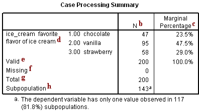
b. N -N provides the number of observations fitting the description in the first column. For example, the first three values give the number of observations for which the subject’s preferred flavor of ice cream is chocolate, vanilla or strawberry, respectively.
c. Marginal Percentage – The marginal percentage lists the proportion of valid observations found in each of the outcome variable’s groups. This can be calculated by dividing the N for each group by the N for “Valid”. Of the 200 subjects with valid data, 47 preferred chocolate ice cream to vanilla and strawberry. Thus, the marginal percentage for this group is (47/200) * 100 = 23.5 %.
d. ice_cream – In this regression, the outcome variable is ice_cream which contains a numeric code for the subject’s favorite flavor of ice cream. The data includes three levels of ice_cream representing three different preferred flavors: 1 = chocolate, 2 = vanilla and 3 = strawberry.
e. Valid – This indicates the number of observations in the dataset where the outcome variable and all predictor variables are non-missing.
f. Missing – This indicates the number of observations in the dataset where data are missing from the outcome variable or any of the predictor variables.
g. Total – This indicates the total number of observations in the dataset–the sum of the number of observations in which data are missing and the number of observations with valid data.
h. Subpopulation – This indicates the number of subpopulations contained in the data. A subpopulation of the data consists of one combination of the predictor variables specified for the model. For example, all records where female = 0, video = 42 and puzzle = 26 would be considered one subpopulation of the data. The footnote SPSS provides indicates how many of these combinations of the predictor variables consist of records that all have the same value in the outcome variable. In this case, there are 143 combinations of female, video and puzzle that appear in the data and 117 of these combinations are composed of records with the same preferred flavor of ice cream.
Model Fitting Information

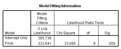
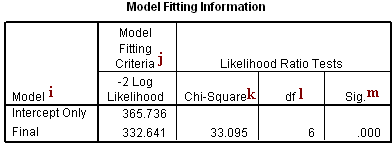
i. Model – This indicates the parameters of the model for which the model fit is calculated. “Intercept Only” describes a model that does not control for any predictor variables and simply fits an intercept to predict the outcome variable. “Final” describes a model that includes the specified predictor variables and has been arrived at through an iterative process that maximizes the log likelihood of the outcomes seen in the outcome variable. By including the predictor variables and maximizing the log likelihood of the outcomes seen in the data, the “Final” model should improve upon the “Intercept Only” model. This can be seen in the differences in the -2(Log Likelihood) values associated with the models.
j. -2(Log Likelihood) – This is the product of -2 and the log likelihoods of the null model and fitted “final” model. The likelihood of the model is used to test of whether all predictors’ regression coefficients in the model are simultaneously zero and in tests of nested models.
k. Chi-Square – This is the Likelihood Ratio (LR) Chi-Square test that at least one of the predictors’ regression coefficient is not equal to zero in the model. The LR Chi-Square statistic can be calculated by -2*L(null model) – (-2*L(fitted model)) = 365.736 – 332.641 = 33.095, where L(null model) is from the log likelihood with just the response variable in the model (Intercept Only) and L(fitted model) is the log likelihood from the final iteration (assuming the model converged) with all the parameters.
l. df – This indicates the degrees of freedom of the chi-square distribution used to test the LR Chi-Sqare statistic and is defined by the number of predictors in the model (three predictors in two models).
m. Sig. – This is the probability getting a LR test statistic being as extreme as, or more so, than the observed statistic under the null hypothesis; the null hypothesis is that all of the regression coefficients in the model are equal to zero. In other words, this is the probability of obtaining this chi-square statistic (33.095), or one more extreme, if there is in fact no effect of the predictor variables. This p-value is compared to a specified alpha level, our willingness to accept a type I error, which is typically set at 0.05 or 0.01. The small p-value from the LR test, <0.00001, would lead us to conclude that at least one of the regression coefficients in the model is not equal to zero. The parameter of the chi-square distribution used to test the null hypothesis is defined by the degrees of freedom in the prior column.
Pseudo R-Square

Pseudo R-Square – These are three pseudo R-squared values. Logistic regression does not have an equivalent to the R-squared that is found in OLS regression; however, many people have tried to come up with one. There are a wide variety of pseudo R-squared statistics which can give contradictory conclusions. Because these statistics do not mean what R-squared means in OLS regression (the proportion of variance of the response variable explained by the predictors), we suggest interpreting them with great caution.
Parameter Estimates

n. B – These are the estimated multinomial logistic regression coefficients for the models. An important feature of the multinomial logit model is that it estimates k-1 models, where k is the number of levels of the outcome variable. In this instance, SPSS is treating the vanilla as the referent group and therefore estimated a model for chocolate relative to vanilla and a model for strawberry relative to vanilla. Therefore, since the parameter estimates are relative to the referent group, the standard interpretation of the multinomial logit is that for a unit change in the predictor variable, the logit of outcome m relative to the referent group is expected to change by its respective parameter estimate (which is in log-odds units) given the variables in the model are held constant.
chocolate relative to vanilla
Intercept – This is the multinomial logit estimate for chocolate relative to vanilla when the predictor variables in the model are evaluated at zero. For males (the variable female evaluated at zero) with zero video and puzzle scores, the logit for preferring chocolate to vanilla is 1.912. Note that evaluating video and puzzle at zero is out of the range of plausible scores, and if the scores were mean-centered, the intercept would have a natural interpretation: log odds of preferring chocolate to vanilla for a male with average video and puzzle scores.
video – This is the multinomial logit estimate for a one unit increase in video score for chocolate relative to vanilla given the other variables in the model are held constant. If a subject were to increase his video score by one point, the multinomial log-odds of preferring chocolate to vanilla would be expected to decrease by 0.024 unit while holding all other variables in the model constant.
puzzle – This is the multinomial logit estimate for a one unit increase in puzzle score for chocolate relative to vanilla given the other variables in the model are held constant. If a subject were to increase his puzzle score by one point, the multinomial log-odds of preferring chocolate to vanilla would be expected to decrease by 0.039 unit while holding all other variables in the model constant.
female – This is the multinomial logit estimate comparing females to males for chocolate relative to vanilla given the other variables in the model are held constant. The multinomial logit for females relative to males is 0.817 unit higher for preferring chocolate relative to vanilla given all other predictor variables in the model are held constant. In other words, females are more likely than males to prefer chocolate ice cream to vanilla ice cream.
strawberry relative to vanilla
Intercept – This is the multinomial logit estimate for strawberry relative to vanilla when the predictor variables in the model are evaluated at zero. For males (the variable female evaluated at zero) with zero video and puzzle scores, the logit for preferring strawberry to vanilla is -4.057.
video – This is the multinomial logit estimate for a one unit increase in video score for strawberry relative to vanilla given the other variables in the model are held constant. If a subject were to increase his video score by one point, the multinomial log-odds for preferring strawberry to vanilla would be expected to increase by 0.023 unit while holding all other variables in the model constant.
puzzle – This is the multinomial logit estimate for a one unit increase in puzzle score for strawberry relative to vanilla given the other variables in the model are held constant. If a subject were to increase his puzzle score by one point, the multinomial log-odds for preferring strawberry to vanilla would be expected to increase by 0.043 unit while holding all other variables in the model constant.
female – This is the multinomial logit estimate comparing females to males for strawberry relative to vanilla given the other variables in the model are held constant. The multinomial logit for females relative to males is 0.033 unit lower for preferring strawberry to vanilla given all other predictor variables in the model are held constant. In other words, males are more likely than females to prefer strawberry ice cream to vanilla ice cream.
o. Std. Error – These are the standard errors of the individual regression coefficients for the two respective models estimated.
p. Wald – This is the Wald chi-square test that tests the null hypothesis that the estimate equals 0.
q. df – This column lists the degrees of freedom for each of the variables included in the model. For each of these variables, the degree of freedom is 1.
r. Sig. – These are the p-values of the coefficients or the probability that, within a given model, the null hypothesis that a particular predictor’s regression coefficient is zero given that the rest of the predictors are in the model. They are based on the Wald test statistics of the predictors, which can be calculated by dividing the square of the predictor’s estimate by the square of its standard error. The probability that a particular Wald test statistic is as extreme as, or more so, than what has been observed under the null hypothesis is defined by the p-value and presented here. In multinomial logistic regression, the interpretation of a parameter estimate’s significance is limited to the model in which the parameter estimate was calculated. For example, the significance of a parameter estimate in the chocolate relative to vanilla model cannot be assumed to hold in the strawberry relative to vanilla model.
chocolate relative to vanilla
For chocolate relative to vanilla, the Wald test statistic for the predictor video is 1.262 with an associated p-value of 0.261. If we set our alpha level to 0.05, we would fail to reject the null hypothesis and conclude that for chocolate relative to vanilla, the regression coefficient for video has not been found to be statistically different from zero given puzzle and female are in the model. For chocolate relative to vanilla, the Wald test statistic for the predictor puzzle is 3.978 with an associated p-value of 0.046. If we again set our alpha level to 0.05, we would reject the null hypothesis and conclude that the regression coefficient for puzzle has been found to be statistically different from zero for chocolate relative to vanilla given that video and female are in the model. For chocolate relative to vanilla, the Wald test statistic for the predictor female 4.362 with an associated p-value of 0.037. If we again set our alpha level to 0.05, we would reject the null hypothesis and conclude that the difference between males and females has been found to be statistically different for chocolate relative to vanilla given that video and female are in the model. For chocolate relative to vanilla, the Wald test statistic for the intercept, Intercept is 2.878 with an associated p-value of 0.090. With an alpha level of 0.05, we would fail to reject the null hypothesis and conclude, a) that the multinomial logit for males (the variable female evaluated at zero) and with zero video and puzzle scores in chocolate relative to vanilla are found not to be statistically different from zero; or b) for males with zero video and puzzle scores, you are statistically uncertain whether they are more likely to be classified as chocolate or vanilla. We can make the second interpretation when we view the Intercept as a specific covariate profile (males with zero video and puzzle scores). Based on the direction and significance of the coefficient, the Intercept indicates whether the profile would have a greater propensity to be classified in one level of the outcome variable than the other level.
strawberry relative to vanilla
For strawberry relative to vanilla, the Wald test statistic for the predictor video is 1.206 with an associated p-value of 0.272. If we set our alpha level to 0.05, we would fail to reject the null hypothesis and conclude that for strawberry relative to vanilla, the regression coefficient for video has not been found to be statistically different from zero given puzzle and female are in the model. For strawberry relative to vanilla, the Wald test statistic for the predictor puzzle is 4.675 with an associated p-value of 0.031. If we again set our alpha level to 0.05, we would reject the null hypothesis and conclude that the regression coefficient for puzzle has been found to be statistically different from zero for strawberry relative to vanilla given that video and female are in the model.
For strawberry relative to vanilla, the Wald test statistic for the predictor female is 0.009 with an associated p-value of 0.925. If we again set our alpha level to 0.05, we would fail to reject the null hypothesis and conclude that for strawberry relative to vanilla, the regression coefficient for female has not been found to be statistically different from zero given puzzle and video are in the model. For strawberry relative to vanilla, the Wald test statistic for the intercept, Intercept is 11.007 with an associated p-value of 0.001. With an alpha level of 0.05, we would reject the null hypothesis and conclude that a) that the multinomial logit for males (the variable female evaluated at zero) and with zero video and puzzle scores in strawberry relative to vanilla are statistically different from zero; or b) for males with zero video and puzzle scores, there is a statistically significant difference between the likelihood of being classified as strawberry or vanilla. We can make the second interpretation when we view the Intercept as a specific covariate profile (males with zero video and puzzle scores). Based on the direction and significance of the coefficient, the Intercept indicates whether the profile would have a greater propensity to be classified in one level of the outcome variable than the other level.
s. Exp(B) – These are the odds ratios for the predictors. They are the exponentiation of the coefficients. There is no odds ratio for the variable ice_cream because ice_cream (as a variable with 2 degrees of freedom) was not entered into the logistic regression equation. The odds ratio of a coefficient indicates how the risk of the outcome falling in the comparison group compared to the risk of the outcome falling in the referent group changes with the variable in question. An odds ratio > 1 indicates that the risk of the outcome falling in the comparison group relative to the risk of the outcome falling in the referent group increases as the variable increases. In other words, the comparison outcome is more likely. An odds ratio < 1 indicates that the risk of the outcome falling in the comparison group relative to the risk of the outcome falling in the referent group decreases as the variable increases. See the interpretations of the relative risk ratios below for examples. In general, if the odds ratio < 1, the outcome is more likely to be in the referent group. For more information on interpreting odds ratios, please see How do I interpret odds ratios in logistic regression? and Understanding RR ratios in multinomial logistic regression .
chocolate relative to vanilla
video – This is the odds or “relative risk” ratio for a one unit increase in video score for chocolate relative to vanilla level given that the other variables in the model are held constant. If a subject were to increase her video score by one unit, the relative risk for preferring chocolate to vanilla would be expected to decrease by a factor of 0.977 given the other variables in the model are held constant. So, given a one unit increase in video, the relative risk of being in the chocolate group would be 0.977 times more likely when the other variables in the model are held constant. More generally, we can say that if a subject were to increase her video score, we would expect her to be more likely to prefer vanilla ice cream over chocolate ice cream.
puzzle – This is the relative risk ratio for a one unit increase in puzzle score for chocolate relative to vanilla level given that the other variables in the model are held constant. If a subject were to increase her puzzle score by one unit, the relative risk for preferring chocolate to vanilla would be expected to decrease by a factor of 0.962 given the other variables in the model are held constant. More generally, we can say that if two subjects have identical video scores and are both female (or both male), the subject with the higher puzzle score is more likely to prefer vanilla ice cream over chocolate ice cream than the subject with the lower puzzle score.
female – This is the relative risk ratio comparing females to males for chocolate relative to vanilla level given that the other variables in the model are held constant. For females relative to males, the relative risk for preferring chocolate relative to vanilla would be expected to increase by a factor of 2.263 given the other variables in the model are held constant. In other words, females are more likely than males to prefer chocolate ice cream over vanilla ice cream.
strawberry relative to vanilla
video – This is the relative risk ratio for a one unit increase in video score for strawberry relative to vanilla level given that the other variables in the model are held constant. If a subject were to increase her video score by one unit, the relative risk for strawberry relative to vanilla would be expected to increase by a factor of 1.023 given the other variables in the model are held constant. More generally, we can say that if a subject were to increase her video score, we would expect her to be more likely to prefer strawberry ice cream over vanilla ice cream.
puzzle – This is the relative risk ratio for a one unit increase in puzzle score for strawberry relative to vanilla level given that the other variables in the model are held constant. If a subject were to increase her puzzle score by one unit, the relative risk for strawberry relative to vanilla would be expected to increase by a factor of 1.044 given the other variables in the model are held constant. More generally, we can say that if two subjects have identical video scores and are both female (or both male), the subject with the higher puzzle score is more likely to prefer strawberry ice cream to vanilla ice cream than the subject with the lower puzzle score.
female – This is the relative risk ratio comparing females to males for strawberry relative to vanilla given that the other variables in the model are held constant. For females relative to males, the relative risk for preferring strawberry to vanilla would be expected to decrease by a factor of 0.968 given the other variables in the model are held constant. In other words, females are less likely than males to prefer strawberry ice cream to vanilla ice cream.
t. 95% Confidence Interval for Exp(B) – This is the Confidence Interval (CI) for an individual multinomial odds ratio given the other predictors are in the model for outcome m relative to the referent group. For a given predictor with a level of 95% confidence, we’d say that we are 95% confident that the “true” population multinomial odds ratio lies between the lower and upper limit of the interval for outcome m relative to the referent group. It is calculated as the Exp(B (zα/2)*(Std.Error)), where zα/2 is a critical value on the standard normal distribution. This CI is equivalent to the z test statistic: if the CI includes one, we’d fail to reject the null hypothesis that a particular regression coefficient is zero given the other predictors are in the model. An advantage of a CI is that it is illustrative; it provides a range where the “true” odds ratio may lie.
