Ordered Logistic Regression
This page shows an example of an ordered logistic regression analysis with footnotes explaining the output. The hsb2 data were collected on 200 high school students with scores on various tests, including science, math, reading and social studies. The outcome measure in this analysis is socio-economic status (ses)- low, medium and high- and the independent variables or predictors include science test scores (science), social science test scores (socst) and gender (female). Our response variable, ses, is going to be treated as ordinal under the assumption that the levels of ses status have a natural ordering (low to high), but the distances between adjacent levels are unknown.
get file = 'C:\data\hsb2.sav'

plum ses with female science socst
/link = logit
/print = parameter summary tparallel.
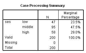


Case Processing Summary
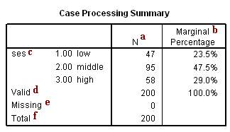
a. N -N provides the number of observations fitting the description from the first column. For example, the first three values give the number of observations for students that report an ses value of low, middle, or high, respectively.
b. Marginal Percentage – The marginal percentage lists the proportion of valid observations found in each of the outcome variable’s groups. This can be calculated by dividing the N for each group by the N for “Valid”. Of the 200 subjects with valid data, 47 were categorized as low ses. Thus, the marginal percentage for this group is (47/200) * 100 = 23.5 %.
c. ses – In this regression, the outcome variable is ses which contains a numeric code for the subject’s socio-economic status. The data includes three levels of ses.
d. Valid – This indicates the number of observations in the dataset where the outcome variable and all predictor variables are non-missing.
e. Missing – This indicates the number of observations in the dataset where data are missing from the outcome variable or any of the predictor variables.
f. Total – This indicates the total number of observations in the dataset–the sum of the number of observations in which data are missing and the number of observations with valid data.
Model Fitting

g. Model – This indicates the parameters of the model for which the model fit is calculated. “Intercept Only” describes a model that does not control for any predictor variables and simply fits an intercept to predict the outcome variable. “Final” describes a model that includes the specified predictor variables whose coefficient have been estimated using an iterative process that maximizes the log likelihood of the outcome. By including the predictor variables and maximizing the log likelihood of the outcome, the “Final” model should improve upon the “Intercept Only” model. This can be seen in the differences in the -2(Log Likelihood) values associated with the models.
h. -2(Log Likelihood) – This is the product of -2 and the log likelihoods of the null model and fitted “final” model. The likelihood of the model is used to test whether all of the estimated regression coefficients in the model are simultaneously zero.
i. Chi-Square – This is the Likelihood Ratio (LR) Chi-Square test. It tests whether at least one of the predictors’ regression coefficient is not equal to zero in the model. The LR Chi-Square statistic can be calculated by -2*L(null model) – (-2*L(fitted model)) = 365.736 – 334.176 = 31.560, where L(null model) is from the log likelihood with just the response variable in the model (Iteration 0) and L(fitted model) is the log likelihood from the final iteration (assuming the model converged) with all the parameters.
j. df – This indicates the degrees of freedom of the Chi-Square distribution used to test the LR Chi-Sqare statistic and is defined by the number of predictors in the model.
k. Sig. – This is the probability of getting a LR test statistic as extreme as, or more so, than the observed under the null hypothesis; the null hypothesis is that all of the regression coefficients in the model are equal to zero. In other words, this is the probability of obtaining this chi-square statistic (31.56) if there is in fact no effect of the predictor variables. This p-value is compared to a specified alpha level, our willingness to accept a type I error, which is typically set at 0.05 or 0.01. The small p-value from the LR test, <0.00001, would lead us to conclude that at least one of the regression coefficients in the model is not equal to zero. The parameter of the Chi-Square distribution used to test the null hypothesis is defined by the degrees of freedom in the prior column.
Pseudo R-Squares
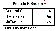
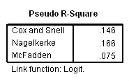
l. Pseudo R-Square – These are three pseudo R-squared values. Logistic regression does not have an equivalent to the R-squared that is found in OLS regression; however, many people have tried to come up with one. There are a wide variety of pseudo R-squared statistics which can give contradictory conclusions. Since these “pseudo” R-squared values do not ave the same interpretation as standard R-squared values from OLS regression (the proportion of variance for the response variable explained by the predictors), we suggest interpreting them with great caution.
Parameter Estimates

m. Threshold – This represents the response variable in the ordered logistic regression. The threshold estimate for [ses = 1.00] is the cutoff value between low and middle ses and the threshold estimate for [ses = 2.00] represents the cutoff value between middle and high ses.
For [ses = 1.00] this is the estimated cutpoint on the latent variable used to differentiate low ses from middle and high ses when values of the predictor variables are evaluated at zero. Subjects that had a value of 2.755 or less on the underlying latent variable that gave rise to our ses variable would be classified as low ses given they were male (the variable female evaluated at zero, its reference value) and had zero science and socst test scores.
[ses = 2.00] – This is the estimated cutpoint on the latent variable used to differentiate low and middle ses from high ses when values of the predictor variables are evaluated at zero. Subjects that had a value of 5.105 or greater on the underlying latent variable that gave rise to our ses variable would be classified as high ses given they were male and had zero science and socst test scores. Subjects that had a value between 2.755 and 5.105 on the underlying latent variable would be classified as middle ses.
n. Estimate – These are the ordered log-odds (logit) regression coefficients. Standard interpretation of the ordered logit coefficient is that for a one unit increase in the predictor, the response variable level is expected to change by its respective regression coefficient in the ordered log-odds scale while the other variables in the model are held constant. Interpretation of the ordered logit estimates is not dependent on the ancillary parameters; the ancillary parameters are used to differentiate the adjacent levels of the response variable. However, since the ordered logit model estimates one equation over all levels of the outcome variable, a concern is whether our one-equation model is valid or if a more flexible model is required. The odds ratios of the predictors can be calculated by exponentiating the estimate.
science – This is the ordered log-odds estimate for a one unit increase in science score on the expected ses level given the other variables are held constant in the model. If a subject were to increase his science score by one point, his ordered log-odds of being in a higher ses category would increase by 0.03 while the other variables in the model are held constant.
socst – This is the ordered log-odds estimate for a one unit increase in socst score on the expected ses level given the other variables are held constant in the model. A one unit increase in socst test scores would result in a 0.053 unit increase in the ordered log-odds of being in a higher ses category while the other variables in the model are held constant.
female – This is the ordered log-odds estimate of comparing females to males on expected ses given the other variables are held constant in the model. The ordered logit for females being in a higher ses category is -0.4824 less than males when the other variables in the model are held constant.
o. Std. Error – These are the standard errors of the individual regression coefficients. They are used in both the calculation of the Wald test statistic, superscript p, and the confidence interval of the regression coefficient, superscript r.
p. Wald – This is the Wald chi-square test that tests the null hypothesis that the estimate equals 0.
q. DF – These are the degrees of freedom for each of the tests of the coefficients. For each Estimate (parameter) estimated in the model, one DF isrequired, and the DF defines the Chi-Square distribution to test whether the individual regression coefficient is zero given the other variables are in the model.
r. Sig.– These are the p-values of the coefficients or the probability that, within a given model, the null hypothesis that a particular predictor’s regression coefficient is zero given that the rest of the predictors are in the model. They are based on the Wald test statistics of the predictors, which can be calculated by dividing the square of the predictor’s estimate by the square of its standard error. The probability that a particular Wald test statistic is as extreme as, or more so, than what has been observed under the null hypothesis is defined by the p-value and presented here. The Wald test statistic for the predictor female is 3.000 with an associated p-value of 0.083. If we set our alpha level to 0.05, we would fail to reject the null hypothesis and conclude that the regression coefficient for female has not been found to be statistically different from zero in estimating ses given socst and science are in the model. The Wald test statistic for the predictor science is 3.584 with an associated p-value of 0.058. If we set our alpha level to 0.05, we would fail to reject the null hypothesis and conclude that the regression coefficient for science has not been found to be statistically different from zero in estimating ses given socst and female are in the model. The Wald test statistic for the predictor socst is 12.777 with an associated p-value of <0.0001. If we again set our alpha level to 0.05, we would reject the null hypothesis and conclude that the regression coefficient for socst has been found to be statistically different from zero in estimating ses given that science and female are in the model. The interpretation for a dichotomous variable such as female, parallels that of a continuous variable: the observed difference between males and females on ses status was not found to be statistically significant at the 0.05 level when controlling for socst and science (p=0.083).
s. 95% Confidence Interval – This is the Confidence Interval (CI) for an individual regression coefficient given the other predictors are in the model. It is calculated as the Coef. (zα/2)*(Std.Err.), where zα/2 is a critical value on the standard normal distribution. The CI is equivalent to the z test statistic: if the CI includes zero, we’d fail to reject the null hypothesis that a particular regression coefficient is zero given the other predictors are in the model.
Test of Parallel Lines
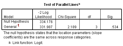
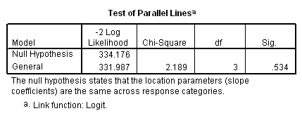
t. General – Here, SPSS tests the proportional odds assumption. This is commonly referred to as the test of parallel lines because the null hypothesis states that the slope coefficients in the model are the same across response categories (and lines of the same slope are parallel). Since the ordered logit model estimates one equation over all levels of the response variable (as compared to the multinomial logit model, which models, assuming low ses is our referent level, an equation for medium ses versus low ses, and an equation for high ses versus low ses), the test for proportional odds tests whether our one-equation model is valid. If we were to reject the null hypothesis based on the significance of the Chi-Square statistic, we would conclude that ordered logit coefficients are not equal across the levels of the outcome, and we would fit a less restrictive model (i.e., multinomial logit model). If we fail to reject the null hypothesis, we conclude that the assumption holds. For our model, the proportional odds assumption appears to have held because our the significance of our Chi-Square statistic is .534 > .05.
