This page shows an example of Poisson regression analysis with footnotes explaining the output in SPSS. The data collected were academic information on 316 students. The response variable is days absent during the school year (daysabs). We explore its relationship with math standardized test scores (mathnce), language standardized test scores (langnce) and gender (female).
As assumed for a Poisson model, our response variable is a count variable, and each subject has the same length of observation time. Had the observation time for subjects varied (i.e., some subjects were followed for half a year, some for a year and the rest for two years) and we were to neglect these differences in exposure time, our Poisson regression estimate would be biased since our model assumes all subjects had the same follow up time. Also, the Poisson model, as compared to other count models (i.e., negative binomial or zero-inflated models), is assumed the appropriate model. In other words, we assume that the response variable is not over-dispersed and does not have an excessive number of zeros.
The dataset can be downloaded here.
get file 'D:\data\lahigh.sav'.
recode gender (1=1) (else = 0) into female.
exe.
In SPSS, Poisson models are treated as a subset of generalized linear models. This is reflected in the syntax. A generalized linear model is Poisson if the specified distribution is Poisson and the link function is log.
genlin daysabs with female mathnce langnce
/model female mathnce langnce distribution = poisson link = log
/print cps history solution fit.
Case Processing Summary
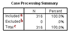
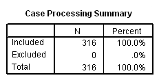
a. Included – This is the number of observations from the dataset included in the model. A observation is included if the outcome variable and all predictor variables have valid, non-missing values.
b. Excluded – This is the number of observations from the dataset not included in the model due to missing data in any of the outcome or predictor variables.
c. Total – This is the sum of the included and excluded records. It is equal to the total number of observations in the dataset.
Iteration History
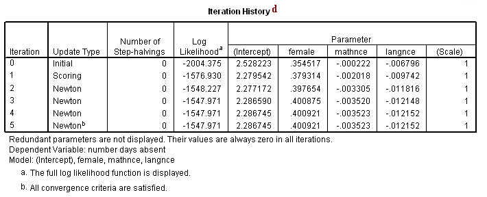
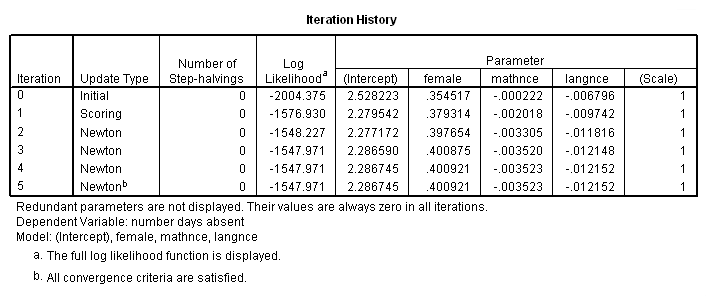
d. Iteration History – This is a listing of the log likelihoods at each iteration. Remember Poisson regression, like binary and ordered logistic regression, uses maximum likelihood estimation, which is an iterative procedure. The first iteration (called iteration 0) is the log likelihood of the “null” model. At each iteration, the log likelihood increases because the goal is to maximize the log likelihood. When the difference between successive iterations is very small, the model is said to have “converged”, the iterating stops, and the results are displayed. For more information on this process for binary outcomes, see Regression Models for Categorical and Limited Dependent Variables by J. Scott Long (page 52-61).
Gradient Vector and Hessian Matrix
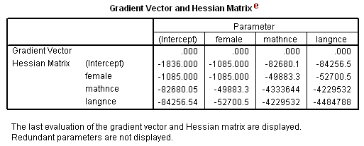
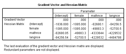
e. Gradient Vector and Hessian Matrix – In our model, we are estimating k+1 parameters where k is the number of predictors: one for each of our predictors and one intercept parameter. The log likelihood of our model is calculated based on these estimated parameters. The gradient vector is the vector of partial derivatives of the log likelihood function with respect to the estimated parameters and the Hessian matrix is the square matrix of second derivatives of this log likelihood with respect to the estimated parameters. The variance-covariance matrix of the model parameters is the negative of the inverse of the Hessian. The values in the Hessian can suggest convergence problems in the model, but the iteration history and possible error messages provided by SPSS are more useful tools in diagnosing problems with the model.
Goodness-of-Fit
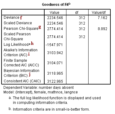
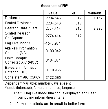
f. Deviance – Deviance is usually defined as the log likelihood of the final model, multiplied by (-2). However, for Poisson regression, SPSS calculates the deviance as
Note that the log likelihood of the model is -1547.971. The usual formulation of the deviance would yield (-2)(-1547.971) = 3095.942, which is greater than the deviance calculated using the above formula.
g. Pearson Chi-Square – This is a goodness-of-fit measure that compares the predicted values of the outcome variable with the actual values. It is calculated as
There is no scaling in this model, so we see that the Scaled Pearson Chi-Square is equal to the Pearson Chi-Square.
h. Log Likelihood – This is the log likelihood of the final model.
i. AIC – This is the Akaike information criterion, a goodness-of-fit measure defined as (–2 ln L + 2k) where k is the number of parameters in the model and L is the likelihood function of the final model.
j. BIC – This is the Bayesian information criterion, a goodness of fit measure defined as
where n is the total number of observations, k is the number of model parameters, and L is the likelihood function of the final model.
Parameter Estimates
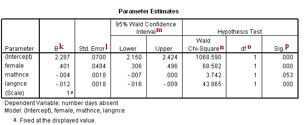
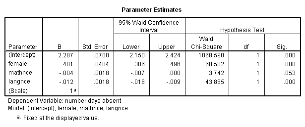
k. B – These are the estimated Poisson regression coefficients for the model. Recall that the response variable is a count variable, and Poisson regression models the log of the expected count as a function of the predictor variables. We can interpret the Poisson regression coefficient as follows: for a one unit change in the predictor variable, the difference in the logs of expected counts is expected to change by the respective regression coefficient, given the other predictor variables in the model are held constant.
(Intercept) – This is the Poisson regression estimate when all variables in the model are evaluated at zero. For males (the variable female evaluated at zero) with zero mathnce and langnce test scores, the log of the expected count for daysabs is 2.287 units. Note that evaluating mathnce and langnce at zero is out of the range of plausible test scores. If the test scores were mean-centered, the intercept would have a natural interpretation: the log of the expected count for males with average mathnce and langnce test scores.
female – This is the estimated Poisson regression coefficient comparing females to males, given the other variables are held constant in the model. The difference in the logs of expected counts is expected to be 0.401 unit higher for females compared to males, while holding the other variables constant in the model. So if we consider two students, one male and one female, with identical math and language test scores, the female student will have a higher predicted value of log(# days absent) than the male student. Thus, we would expect the female student to have more days absent than her male counterpart.
mathnce – This is the Poisson regression estimate for a one unit increase in math standardized test score, given the other variables are held constant in the model. If a student were to increase her mathnce test score by one point, the difference in the logs of expected counts would be expected to decrease by 0.004 unit, while holding the other variables in the model constant. If we consider two students of the same sex who have the same language score, we would expect the student with the higher math score of the two to have fewer days absent than the other student.
langnce – This is the Poisson regression estimate for a one unit increase in language standardized test score, given the other variables are held constant in the model. If a student were to increase her langnce test score by one point, the difference in the logs of expected counts would be expected to decrease by 0.012 unit while holding the other variables in the model constant. If we consider two students of the same sex who have the same math score, we would expect the student with the higher language score of the two to have fewer days absent than the other student.
l. Std. Error – These are the standard errors of the individual regression coefficients. They are used both in the calculation of the Wald Chi-Square test statistic, superscript l, and the confidence interval of the regression coefficient, superscript k.
m. 95% Wald Confidence Interval – This is the confidence interval (CI) of an individual Poisson regression coefficient, given the other predictors are in the model. For a given predictor variable with a level of 95% confidence, we’d say that we are 95% confident that upon repeated trials 95% of the CI’s would include the “true” population Poisson regression coefficient. It is calculated as B (zα/2)*(Std.Error), where zα/2 is a critical value on the standard normal distribution. The CI is equivalent to the z test statistic: if the CI includes zero, we’d fail to reject the null hypothesis that a particular regression coefficient is zero, given the other predictors are in the model. An advantage of a CI is that it is illustrative; it provides information on where the “true” parameter may lie and the precision of the point estimate.
n. Wald Chi-Square – These are the test statistics for the individual regression coefficients. The test statistic is the squared ratio of the coefficient B to the Std. Error of the respective predictor. The test statistic follows a Chi-Square distribution which is used to test against a two-sided alternative hypothesis that the B is not equal to zero.
o. df – This column lists the degrees of freedom for each of the variables included in the model. For each of these variables, the degree of freedom is 1.
p. Sig. – These are the p-values of the coefficients or the probability that, within a given model, the null hypothesis that a particular predictor’s regression coefficient is zero given that the rest of the predictors are in the model. They are based on the Wald Chi-Square test statistics of the predictors. The probability that a particular Wald test statistic is as extreme as, or more so, than what has been observed under the null hypothesis is defined by the p-value and presented here. By looking at the estimates of the standard errors to a greater degree of precision, we can calculate the test statistics and see that they match those produced in SPSS. To view the estimates with more decimal places displayed, click on the Parameter Estimates table in your SPSS output, then double-click on the number of interest.
(Intercept) – The Wald Chi-Square test statistic testing (Intercept) is zero, given the other variables are in the model and evaluated at zero, is (2.286745/ 0.0699539)2 = 1068.590, with an associated p-value of <0.0001. If we set our alpha level at 0.05, we would reject the null hypothesis and conclude that (Intercept) on daysabs has been found to be statistically different from zero given mathnce, langnce and female are in the model and evaluated at zero.
female – The Wald Chi-Square test statistic testing the difference between the log of expected counts between males and females on daysabs is zero, given the other variables are in the model, is (0.4009209/0.0484122)2= 68.582, with an associated p-value of <0.0001. If we set our alpha level at 0.05, we would reject the null hypothesis and conclude that the coefficient for female is statistically different from zero given mathnce and langnce are in the model.
mathnce – The Wald Chi-Square test statistic testing the slope for mathnce on daysabs is zero, given the other variables are in the model, is (-0.0035232/0.0018213)2 = 3.742, with an associated p-value of 0.053. If we set our alpha level at 0.05, we would fail to reject the null hypothesis and conclude the poisson regression coefficient for mathnce is not statistically different from zero given langnce and female are in the model.
langnce – The Wald Chi-Square test statistic testing the slope for langnce on daysabs is zero, given the other variables are in the model, is (-0.0121521/0.0018348)2 = 43.865, with an associated p-value of <0.0001. If we set our alpha level at 0.05, we would reject the null hypothesis and conclude the poisson regression coefficient for langnce is statistically different from zero given mathnce and female are in the model.


