This page shows an example of a principal components analysis with footnotes explaining the output. The data used in this example were collected by Professor James Sidanius, who has generously shared them with us. You can download the data set here.
Overview: The “what” and “why” of principal components analysis
Principal components analysis is a method of data reduction. Suppose that you have a dozen variables that are correlated. You might use principal components analysis to reduce your 12 measures to a few principal components. In this example, you may be most interested in obtaining the component scores (which are variables that are added to your data set) and/or to look at the dimensionality of the data. For example, if two components are extracted and those two components accounted for 68% of the total variance, then we would say that two dimensions in the component space account for 68% of the variance. Unlike factor analysis, principal components analysis is not usually used to identify underlying latent variables. Hence, the loadings onto the components are not interpreted as factors in a factor analysis would be. Principal components analysis, like factor analysis, can be preformed on raw data, as shown in this example, or on a correlation or a covariance matrix. If raw data are used, the procedure will create the original correlation matrix or covariance matrix, as specified by the user. If the correlation matrix is used, the variables are standardized and the total variance will equal the number of variables used in the analysis (because each standardized variable has a variance equal to 1). If the covariance matrix is used, the variables will remain in their original metric. However, one must take care to use variables whose variances and scales are similar. Unlike factor analysis, which analyzes the common variance, the original matrix in a principal components analysis analyzes the total variance. Also, principal components analysis assumes that each original measure is collected without measurement error.
Principal components analysis is a technique that requires a large sample size. Principal components analysis is based on the correlation matrix of the variables involved, and correlations usually need a large sample size before they stabilize. Tabachnick and Fidell (2001, page 588) cite Comrey and Lee’s (1992) advise regarding sample size: 50 cases is very poor, 100 is poor, 200 is fair, 300 is good, 500 is very good, and 1000 or more is excellent. As a rule of thumb, a bare minimum of 10 observations per variable is necessary to avoid computational difficulties.
In this example we have included many options, including the original and reproduced correlation matrix and the scree plot. While you may not wish to use all of these options, we have included them here to aid in the explanation of the analysis. We have also created a page of annotated output for a factor analysis that parallels this analysis. For general information regarding the similarities and differences between principal components analysis and factor analysis, see Tabachnick and Fidell (2001), for example.
get data "D:\data\M255.sav".
factor
 /variables item13 item14 item15 item16 item17 item18 item19 item20 item21 item22 item23 item24
 /print initial correlation det kmo repr extraction univariate
 /format blank(.30)
 /plot eigen
 /extraction pc
 /method = correlate.
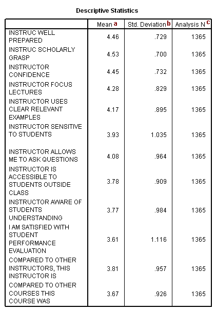
The table above is output because we used the univariate option on the /print subcommand. Please note that the only way to see how many cases were actually used in the principal components analysis is to include the univariate option on the /print subcommand. The number of cases used in the analysis will be less than the total number of cases in the data file if there are missing values on any of the variables used in the principal components analysis, because, by default, SPSS does a listwise deletion of incomplete cases. If the principal components analysis is being conducted on the correlations (as opposed to the covariances), it is not much of a concern that the variables have very different means and/or standard deviations (which is often the case when variables are measured on different scales).
a. Mean – These are the means of the variables used in the factor analysis.
b. Std. Deviation – These are the standard deviations of the variables used in the factor analysis.
c. Analysis N – This is the number of cases used in the factor analysis.
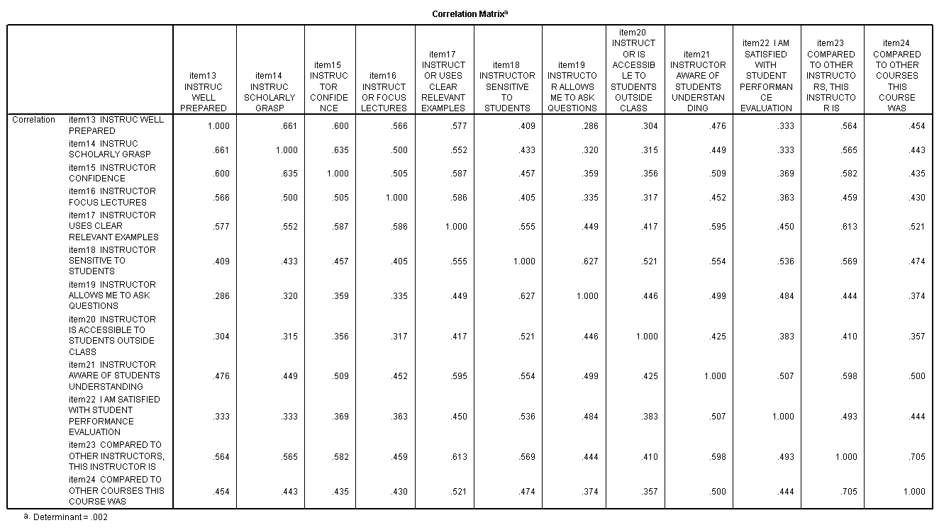
The table above was included in the output because we included the keyword correlation on the /print subcommand. This table gives the correlations between the original variables (which are specified on the /variables subcommand). Before conducting a principal components analysis, you want to check the correlations between the variables. If any of the correlations are too high (say above .9), you may need to remove one of the variables from the analysis, as the two variables seem to be measuring the same thing. Another alternative would be to combine the variables in some way (perhaps by taking the average). If the correlations are too low, say below .1, then one or more of the variables might load only onto one principal component (in other words, make its own principal component). This is not helpful, as the whole point of the analysis is to reduce the number of items (variables).
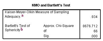
a. Kaiser-Meyer-Olkin Measure of Sampling Adequacy – This measure varies between 0 and 1, and values closer to 1 are better. A value of .6 is a suggested minimum.
b. Bartlett’s Test of Sphericity – This tests the null hypothesis that the correlation matrix is an identity matrix. An identity matrix is matrix in which all of the diagonal elements are 1 and all off diagonal elements are 0. You want to reject this null hypothesis.
Taken together, these tests provide a minimum standard which should be passed before a principal components analysis (or a factor analysis) should be conducted.
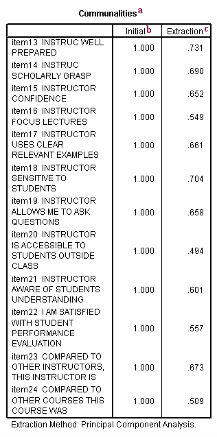
a. Communalities – This is the proportion of each variable’s variance that can be explained by the principal components (e.g., the underlying latent continua). It is also noted as h2 and can be defined as the sum of squared factor loadings.
b. Initial – By definition, the initial value of the communality in a principal components analysis is 1.
c. Extraction – The values in this column indicate the proportion of each variable’s variance that can be explained by the principal components. Variables with high values are well represented in the common factor space, while variables with low values are not well represented. (In this example, we don’t have any particularly low values.) They are the reproduced variances from the number of components that you have saved. You can find these values on the diagonal of the reproduced correlation matrix.
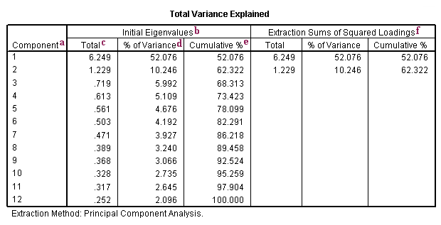
a. Component – There are as many components extracted during a principal components analysis as there are variables that are put into it. In our example, we used 12 variables (item13 through item24), so we have 12 components.
b. Initial Eigenvalues – Eigenvalues are the variances of the principal components. Because we conducted our principal components analysis on the correlation matrix, the variables are standardized, which means that the each variable has a variance of 1, and the total variance is equal to the number of variables used in the analysis, in this case, 12.
c. Total – This column contains the eigenvalues. The first component will always account for the most variance (and hence have the highest eigenvalue), and the next component will account for as much of the left over variance as it can, and so on. Hence, each successive component will account for less and less variance.
d. % of Variance – This column contains the percent of variance accounted for by each principal component.
e. Cumulative % – This column contains the cumulative percentage of variance accounted for by the current and all preceding principal components. For example, the third row shows a value of 68.313. This means that the first three components together account for 68.313% of the total variance. (Remember that because this is principal components analysis, all variance is considered to be true and common variance. In other words, the variables are assumed to be measured without error, so there is no error variance.)
f. Extraction Sums of Squared Loadings – The three columns of this half of the table exactly reproduce the values given on the same row on the left side of the table. The number of rows reproduced on the right side of the table is determined by the number of principal components whose eigenvalues are 1 or greater.
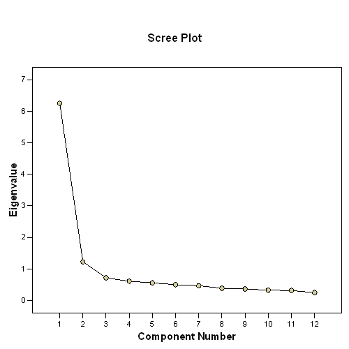
The scree plot graphs the eigenvalue against the component number. You can see these values in the first two columns of the table immediately above. From the third component on, you can see that the line is almost flat, meaning the each successive component is accounting for smaller and smaller amounts of the total variance. In general, we are interested in keeping only those principal components whose eigenvalues are greater than 1. Components with an eigenvalue of less than 1 account for less variance than did the original variable (which had a variance of 1), and so are of little use. Hence, you can see that the point of principal components analysis is to redistribute the variance in the correlation matrix (using the method of eigenvalue decomposition) to redistribute the variance to first components extracted.
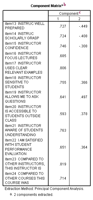
b. Component Matrix – This table contains component loadings, which are the correlations between the variable and the component. Because these are correlations, possible values range from -1 to +1. On the /format subcommand, we used the option blank(.30), which tells SPSS not to print any of the correlations that are .3 or less. This makes the output easier to read by removing the clutter of low correlations that are probably not meaningful anyway.
c. Component – The columns under this heading are the principal components that have been extracted. As you can see by the footnote provided by SPSS (a.), two components were extracted (the two components that had an eigenvalue greater than 1). You usually do not try to interpret the components the way that you would factors that have been extracted from a factor analysis. Rather, most people are interested in the component scores, which are used for data reduction (as opposed to factor analysis where you are looking for underlying latent continua). You can save the component scores to your data set for use in other analyses using the /save subcommand.
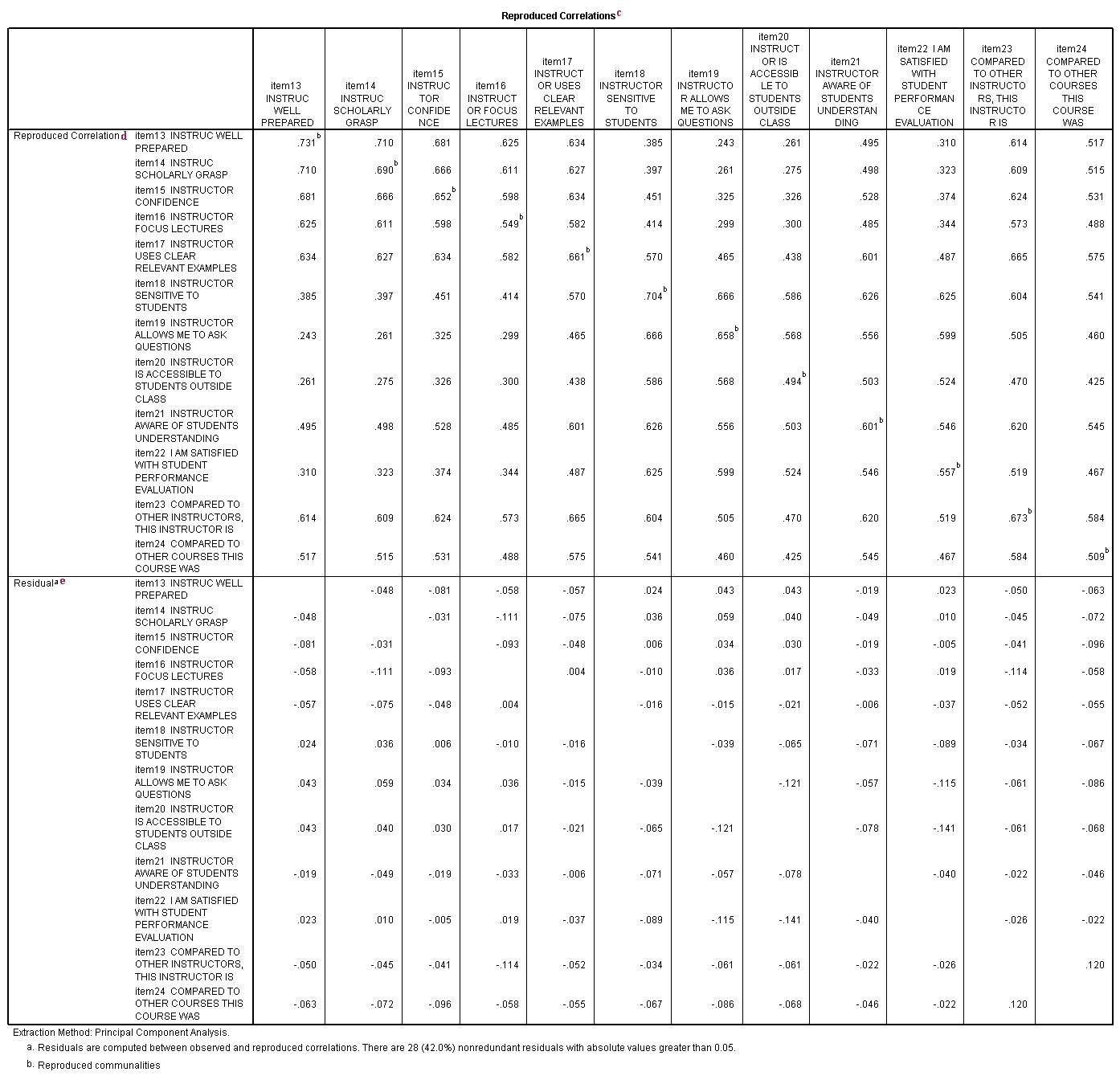
c. Reproduced Correlations – This table contains two tables, the reproduced correlations in the top part of the table, and the residuals in the bottom part of the table.
d. Reproduced Correlation – The reproduced correlation matrix is the correlation matrix based on the extracted components. You want the values in the reproduced matrix to be as close to the values in the original correlation matrix as possible. This means that you want the residual matrix, which contains the differences between the original and the reproduced matrix, to be close to zero. If the reproduced matrix is very similar to the original correlation matrix, then you know that the components that were extracted accounted for a great deal of the variance in the original correlation matrix, and these few components do a good job of representing the original data. The numbers on the diagonal of the reproduced correlation matrix are presented in the Communalities table in the column labeled Extracted.
e. Residual – As noted in the first footnote provided by SPSS (a.), the values in this part of the table represent the differences between original correlations (shown in the correlation table at the beginning of the output) and the reproduced correlations, which are shown in the top part of this table. For example, the original correlation between item13 and item14 is .661, and the reproduced correlation between these two variables is .710. The residual is -.048 = .661 – .710 (with some rounding error).

