This page shows an example of probit regression analysis with footnotes explaining the output in SPSS. The data in this example were gathered on undergraduates applying to graduate school and includes undergraduate GPAs, the reputation of the school of the undergraduate (a topnotch indicator), the students’ GRE score, and whether or not the student was admitted to graduate school. Using this dataset ( https://stats.idre.ucla.edu/wp-content/uploads/2016/02/probit.sav ), we can predict admission to graduate school using undergraduate GPA, GRE scores, and the reputation of the school of the undergraduate. Our outcome variable is binary, and we will use a probit model. Thus, our model will calculate a predicted probability of admission based on our predictors. The probit model does so using the cumulative distribution function of the standard normal.
First, let us examine the dataset and our response variable. Our binary outcome variable must be coded with zeros and ones, so we will include a frequency of our outcome variable admit to check this.
get file='C:\data\probit.sav'.

descriptives
  variables=gre gpa.

frequencies
  variables=admit topnotch.


Next, we can specify our probit model using the plum command and indicating probit as our link function.
plum admit with gre topnotch gpa
/link = probit
/print = parameter summary.


NOTE: It is also possible to run this probit regression in SPSS using genlin. Please note that distribution and link are options on the /model subcommand and are not separate subcommands (which is why there is no / in front of them).
genlin admit (reference=0) with gre gpa topnotch
/model gre gpa topnotch
distribution=binomial
link=probit
/print cps history fit solution.
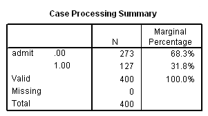
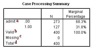
Case Processing Summary

a. admit – This is the response variable predicted by the model. Here, we see that our outcome variable is binary and we are provided with frequency counts. With our model, we predict the probability that admit is 1 for an observation given the values of the predictors.
b. Valid – This is the number of observations in our dataset with valid and non-missing data in the response and predictor variables specified in our model.
c. Missing – This is the number of observations in our dataset with missing data in the response or predictor variables specified in our model. Such observations will be excluded from the analysis.
d. Total – This is the total of the number of valid observations and missing observations. It is equal to the number of observations in the dataset.
Model Fitting Information

e. Model – This indicates the parameters of the model for which the model fit is calculated. “Intercept Only” describes a model that does not control for any predictor variables and simply fits an intercept to predict the outcome variable. “Final” describes a model that includes the specified predictor variables and has been arrived at through an iterative process that maximizes the log likelihood of the outcomes seen in the outcome variable. By including the predictor variables and maximizing the log likelihood of the outcomes seen in the data, the “Final” model should improve upon the “Intercept Only” model. This can be seen in the differences in the -2 Log Likelihood values associated with the models (see superscript f).
f. -2 Log Likelihood – This is the product of -2 and the log likelihoods of the null model and fitted “final” model. The likelihood of the model is used to test of whether all predictors’ regression coefficients in the model are simultaneously zero and in tests of nested models.
g. Chi-Square – This is the Likelihood Ratio (LR) Chi-Square test that at least one of the predictors’ regression coefficient is not equal to zero in the model. The LR Chi-Square statistic can be calculated by -2*L(null model) – (-2*L(fitted model)) = 479.887 – 457.797 = 22.090, where L(null model) is from the log likelihood with just the response variable in the model (Iteration 0) and L(fitted model) is the log likelihood from the final iteration (assuming the model converged) with all the parameters.
h. df – This indicates the degrees of freedom of the Chi-Square distribution used to test the LR Chi-Sqare statistic and is defined by the number of predictors in the model.
i. Sig. – This is the probability of getting a LR test statistic as extreme as, or more so, than the observed under the null hypothesis; the null hypothesis is that all of the regression coefficients in the model are equal to zero. In other words, this is the probability of obtaining this chi-square statistic (22.090) if there is in fact no effect of the predictor variables. This p-value is compared to a specified alpha level, our willingness to accept a type I error, which is typically set at 0.05 or 0.01. The small p-value from the LR test, <0.0001, would lead us to conclude that at least one of the regression coefficients in the model is not equal to zero. The parameter of the Chi-Square distribution used to test the null hypothesis is defined by the degrees of freedom in the prior column.
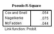
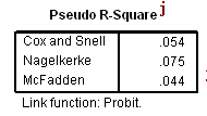
Pseudo R-Square

j. Psuedo R-Square – These are several Pseudo R-Squareds. Probit regression does not have an equivalent to the R-squared that is found in OLS regression; however, many people have tried to come up with one. There are a wide variety of pseudo-R-square statistics. Because these statistics do not mean what R-square means in OLS regression (the proportion of variance of the response variable explained by the predictors), we suggest interpreting these statistics with great caution. For more information on pseudo R-squareds, see What are Pseudo R-Squareds?.
Parameter Estimates

k. Estimate – These are the regression coefficients. The predicted probability of admission can be calculated using these coefficients (the first number in the column, the coefficient for “Threshold” is the constant term in the model). For a given record, the predicted probability of admission is
![]()
where F is the cumulative distribution function of the standard normal. However, interpretation of the coefficients in probit regression is not as straightforward as the interpretations of coefficients in linear regression or logit regression. The increase in probability attributed to a one-unit increase in a given predictor is dependent both on the values of the other predictors and the starting value of the given predictors. For example, if we hold gre and topnotch constant at zero, the one unit increase in gpa from 2 to 3 has a different effect than the one unit increase from 3 to 4 (note that the probabilities do not change by a common difference or common factor):

and the effects of these one unit increases are different if we hold gre and topnotch constant at their respective means instead of zero:

However, there are limited ways in which we can interpret the individual regression coefficients. A positive coefficient mean that an increase in the predictor leads to an increase in the predicted probability. A negative coefficient means that an increase in the predictor leads to a decrease in the predicted probability.
gre – The coefficient of gre is 0.002. This means that an increase in GRE score increases the predicted probability of admission.
topnotch – The coefficient of topnotch is 0.273. This means attending a top notch institution as an undergraduate increases the predicted probability of admission.
gpa – The coefficient of gpa is 0.401. This means that an increase in GPA increases the predicted probability of admission.
Threshold [admit= .00]– This is the constant term in the model. The constant term is -2.798. This means that if all of the predictors (gre, topnotch and gpa) are evaluated at zero, the predicted probability of admission is F(-2.798) = .00257101. So, as expected, the predicted probability of a student with a GRE score of zero and a GPA of zero from a non-topnotch school has an extremely low predicted probability of admission.
l. Std. Error – These are the standard errors of the individual regression coefficients. They are used both in the calculation of the Wald test statistic, superscript m, and the confidence interval of the regression coefficient, superscript m.
m. Wald – These are the test statistics for the individual regression coefficients. The test statistic is the squared ratio of the regression coefficient Estimate to the Std. Error of the respective predictor. The test statistic follows a Chi-Square distribution which is used to test against a two-sided alternative hypothesis that the Estimate is not equal to zero.
n. df – This column lists the degrees of freedom for each of the variables included in the model. For each of these variables, the degree of freedom is 1.
o. Sig. – These are the p-values of the coefficients or the probability that, within a given model, the null hypothesis that a particular predictor’s regression coefficient is zero given that the rest of the predictors are in the model. They are based on the Wald test statistics of the predictors. The probability that a particular Wald test statistic is as extreme as, or more so, than what has been observed under the null hypothesis is defined by the p-value and presented here. By looking at the estimates of the standard errors to a greater degree of precision, we can calculate the test statistics and see that they match those produced in SPSS. To view the estimates with more decimal places displayed, click on the Parameter Estimates table in your SPSS output, then double-click on the number of interest.
The Wald test statistic for the Threshold is 18.664 with an associated p-value <.0001. If we set our alpha level to 0.05, we would reject the null hypothesis and conclude that the model intercept has been found to be statistically different from zero given gre, gpa and topnotch are in the model.
The Wald test statistic for the predictor gre is 5.667 with an associated p-value of 0.017. If we set our alpha level to 0.05, we would reject the null hypothesis and conclude that the regression coefficient for gre has been found to be statistically different from zero in estimating gre given topnotch and gpa are in the model.
The Wald test statistic for the predictor topnotch is 2.292 with an associated p-value of 0.130. If we set our alpha level to 0.05, we would fail to reject the null hypothesis and conclude that the regression coefficient for topnotch has not been found to be statistically different from zero in estimating topnotch given gre and gpa are in the model.
The Wald test statistic for the predictor gpa is 4.237 with an associated p-value of 0.040. If we set our alpha level to 0.05, we would reject the null hypothesis and conclude that the regression coefficient for gpa has been found to be statistically different from zero in estimating gpa given topnotch and gre are in the model.
p. 95% Wald Confidence Interval – This is the confidence interval (CI) of an individual poisson regression coefficient, given the other predictors are in the model. For a given predictor variable with a level of 95% confidence, we’d say that we are 95% confident that upon repeated trials 95% of the CI’s would include the “true” population poisson regression coefficient. It is calculated as B (zα/2)*(Std.Error), where zα/2 is a critical value on the standard normal distribution. The CI is equivalent to the z test statistic: if the CI includes zero, we’d fail to reject the null hypothesis that a particular regression coefficient is zero, given the other predictors are in the model. An advantage of a CI is that it is illustrative; it provides information on where the “true” parameter may lie and the precision of the point estimate.
