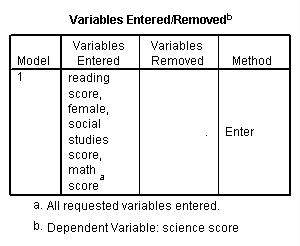
This page shows an example regression analysis with footnotes explaining the output. These data (hsb2) were collected on 200 high schools students and are scores on various tests, including science, math, reading and social studies (socst). The variable female is a dichotomous variable coded 1 if the student was female and 0 if male.
In the syntax below, the get file command is used to load the data into SPSS. In quotes, you need to specify where the data file is located on your computer. Remember that you need to use the .sav extension and that you need to end the command with a period. In the regression command, the statistics subcommand must come before the dependent subcommand. You can shorten dependent to dep. You list the independent variables after the equals sign on the method subcommand. The statistics subcommand is not needed to run the regression, but on it we can specify options that we would like to have included in the output. Here, we have specified ci, which is short for confidence intervals. These are very useful for interpreting the output, as we will see. There are four tables given in the output. SPSS has provided some superscripts (a, b, etc.) to assist you in understanding the output.
Please note that SPSS sometimes includes footnotes as part of the output. We have left those intact and have started ours with the next letter of the alphabet.
get file "c:\data\hsb2.sav".

regression
 /statistics coeff outs r anova ci
 /dependent science
 /method = enter math female socst read.


Variables in the model

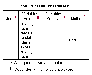
c. Model – SPSS allows you to specify multiple models in a single regression command. This tells you the number of the model being reported.
d. Variables Entered – SPSS allows you to enter variables into a regression in blocks, and it allows stepwise regression. Hence, you need to know which variables were entered into the current regression. If you did not block your independent variables or use stepwise regression, this column should list all of the independent variables that you specified.
e. Variables Removed – This column listed the variables that were removed from the current regression. Usually, this column will be empty unless you did a stepwise regression.
f. Method – This column tells you the method that SPSS used to run the regression. “Enter” means that each independent variable was entered in usual fashion. If you did a stepwise regression, the entry in this column would tell you that.
Overall Model Fit

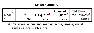
b. Model – SPSS allows you to specify multiple models in a single regression command. This tells you the number of the model being reported.
c. R – R is the square root of R-Squared and is the correlation between the observed and predicted values of dependent variable.
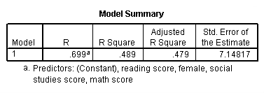
d. R-Square – R-Square is the proportion of variance in the dependent variable (science) which can be predicted from the independent variables (math, female, socst and read). This value indicates that 48.9% of the variance in science scores can be predicted from the variables math, female, socst and read. Note that this is an overall measure of the strength of association, and does not reflect the extent to which any particular independent variable is associated with the dependent variable. R-Square is also called the coefficient of determination.
e. Adjusted R-square – As predictors are added to the model, each predictor will explain some of the variance in the dependent variable simply due to chance. One could continue to add predictors to the model which would continue to improve the ability of the predictors to explain the dependent variable, although some of this increase in R-square would be simply due to chance variation in that particular sample. The adjusted R-square attempts to yield a more honest value to estimate the R-squared for the population. The value of R-square was .489, while the value of Adjusted R-square was .479 Adjusted R-squared is computed using the formula 1 – ((1 – Rsq)(N – 1 )/ (N – k – 1)). From this formula, you can see that when the number of observations is small and the number of predictors is large, there will be a much greater difference between R-square and adjusted R-square (because the ratio of (N – 1) / (N – k – 1) will be much greater than 1). By contrast, when the number of observations is very large compared to the number of predictors, the value of R-square and adjusted R-square will be much closer because the ratio of (N – 1)/(N – k – 1) will approach 1.
f. Std. Error of the Estimate – The standard error of the estimate, also called the root mean square error, is the standard deviation of the error term, and is the square root of the Mean Square Residual (or Error).
Anova Table

c. Model – SPSS allows you to specify multiple models in a single regression command. This tells you the number of the model being reported.
d. This is the source of variance, Regression, Residual and Total. The Total variance is partitioned into the variance which can be explained by the independent variables (Regression) and the variance which is not explained by the independent variables (Residual, sometimes called Error). Note that the Sums of Squares for the Regression and Residual add up to the Total, reflecting the fact that the Total is partitioned into Regression and Residual variance.
e. Sum of Squares – These are the Sum of Squares associated with the three sources of variance, Total, Model and Residual. These can be computed in many ways. Conceptually, these formulas can be expressed as: SSTotal The total variability around the mean. S(Y – Ybar)2. SSResidual The sum of squared errors in prediction. S(Y – Ypredicted)2. SSRegression The improvement in prediction by using the predicted value of Y over just using the mean of Y. Hence, this would be the squared differences between the predicted value of Y and the mean of Y, S(Ypredicted – Ybar)2. Another way to think of this is the SSRegression is SSTotal – SSResidual. Note that the SSTotal = SSRegression + SSResidual. Note that SSRegression / SSTotal is equal to .489, the value of R-Square. This is because R-Square is the proportion of the variance explained by the independent variables, hence can be computed by SSRegression / SSTotal.
f. df – These are the degrees of freedom associated with the sources of variance. The total variance has N-1 degrees of freedom. In this case, there were N=200 students, so the DF for total is 199. The model degrees of freedom corresponds to the number of predictors minus 1 (K-1). You may think this would be 4-1 (since there were 4 independent variables in the model, math, female, socst and read). But, the intercept is automatically included in the model (unless you explicitly omit the intercept). Including the intercept, there are 5 predictors, so the model has 5-1=4 degrees of freedom. The Residual degrees of freedom is the DF total minus the DF model, 199 – 4 is 195.
g. Mean Square – These are the Mean Squares, the Sum of Squares divided by their respective DF. For the Regression,
9543.72074 / 4 = 2385.93019. For the Residual, 9963.77926 / 195 =
51.0963039. These are computed so you can compute the F ratio, dividing the Mean Square Regression by the Mean Square Residual to test the significance of the predictors in the model.
h. F and Sig. – The F-value is the Mean Square Regression (2385.93019) divided by the Mean Square Residual (51.0963039), yielding F=46.69. The p-value associated with this F value is very small (0.0000). These values are used to answer the question “Do the independent variables reliably predict the dependent variable?”. The p-value is compared to your alpha level (typically 0.05) and, if smaller, you can conclude “Yes, the independent variables reliably predict the dependent variable”. You could say that the group of variables math, and female, socst and read can be used to reliably predict science (the dependent variable). If the p-value were greater than 0.05, you would say that the group of independent variables does not show a statistically significant relationship with the dependent variable, or that the group of independent variables does not reliably predict the dependent variable. Note that this is an overall significance test assessing whether the group of independent variables when used together reliably predict the dependent variable, and does not address the ability of any of the particular independent variables to predict the dependent variable. The ability of each individual independent variable to predict the dependent variable is addressed in the table below where each of the individual variables are listed.
Parameter Estimates

b. Model – SPSS allows you to specify multiple models in a single regression command. This tells you the number of the model being reported.
c. This column shows the predictor variables (constant, math, female, socst, read). The first variable (constant) represents the constant, also referred to in textbooks as the Y intercept, the height of the regression line when it crosses the Y axis. In other words, this is the predicted value of science when all other variables are 0.
d. B – These are the values for the regression equation for predicting the dependent variable from the independent variable. These are called unstandardized coefficients because they are measured in their natural units. As such, the coefficients cannot be compared with one another to determine which one is more influential in the model, because they can be measured on different scales. For example, how can you compare the values for gender with the values for reading scores? The regression equation can be presented in many different ways, for example:
Ypredicted = b0 + b1*x1 + b2*x2 + b3*x3 + b3*x3 + b4*x4
The column of estimates (coefficients or parameter estimates, from here on labeled coefficients) provides the values for b0, b1, b2, b3 and b4 for this equation. Expressed in terms of the variables used in this example, the regression equation is
sciencePredicted = 12.325 +
.389*math + -2.010*female+.050*socst+.335*read
These estimates tell you about the relationship between the independent variables and the dependent variable. These estimates tell the amount of increase in science scores that would be predicted by a 1 unit increase in the predictor. Note: For the independent variables which are not significant, the coefficients are not significantly different from 0, which should be taken into account when interpreting the coefficients. (See the columns with the t-value and p-value about testing whether the coefficients are significant). math – The coefficient (parameter estimate) is
.389. So, for every unit (i.e., point, since this is the metric in which the tests are measured) increase in math, a .389 unit increase in science is predicted, holding all other variables constant. (It does not matter at what value you hold the other variables constant, because it is a linear model.) Or, for every increase of one point on the math test, your science score is predicted to be higher by .389 points. This is significantly different from 0. female – For every unit increase in female, there is a
-2.010 unit decrease in the predicted science score, holding all other variables constant. Since female is coded 0/1 (0=male, 1=female) the interpretation can be put more simply. For females the predicted science score would be 2 points lower than for males. The variable female is technically not statistically significantly different from 0, because the p-value is greater than .05. However, .051 is so close to .05 that some researchers would still consider it to be statistically significant. socst – The coefficient for socst is .050. This means that for a 1-unit increase in the social studies score, we expect an approximately .05 point increase in the science score. This is not statistically significant; in other words, .050 is not different from 0. read – The coefficient for read is .335. Hence, for every unit increase in reading score we expect a .335 point increase in the science score. This is statistically significant.
e. Std. Error – These are the standard errors associated with the coefficients. The standard error is used for testing whether the parameter is significantly different from 0 by dividing the parameter estimate by the standard error to obtain a t-value (see the column with t-values and p-values). The standard errors can also be used to form a confidence interval for the parameter, as shown in the last two columns of this table.
f. Beta – These are the standardized coefficients. These are the coefficients that you would obtain if you standardized all of the variables in the regression, including the dependent and all of the independent variables, and ran the regression. By standardizing the variables before running the regression, you have put all of the variables on the same scale, and you can compare the magnitude of the coefficients to see which one has more of an effect. You will also notice that the larger betas are associated with the larger t-values.
g. t and Sig. – These columns provide the t-value and 2 tailed p-value used in testing the null hypothesis that the coefficient/parameter is 0. If you use a 2 tailed test, then you would compare each p-value to your preselected value of alpha. Coefficients having p-values less than alpha are statistically significant. For example, if you chose alpha to be 0.05, coefficients having a p-value of 0.05 or less would be statistically significant (i.e., you can reject the null hypothesis and say that the coefficient is significantly different from 0). If you use a 1 tailed test (i.e., you predict that the parameter will go in a particular direction), then you can divide the p-value by 2 before comparing it to your preselected alpha level. With a 2-tailed test and alpha of 0.05, you should not reject the null hypothesis that the coefficient for female is equal to 0, because p-value = 0.051 > 0.05. The coefficient of -2.009765 is not significantly different from 0. However, if you hypothesized specifically that males had higher scores than females (a 1-tailed test) and used an alpha of 0.05, the p-value of .0255 is less than 0.05 and the coefficient for female would be significant at the 0.05 level. In this case, we could say that the female coefficient is significantly greater than 0. Neither a 1-tailed nor 2-tailed test would be significant at alpha of 0.01.
The constant is significantly different from 0 at the 0.05 alpha level. However, having a significant intercept is seldom interesting.
The coefficient for math (.389) is statistically significantly different from 0 using alpha of 0.05 because its p-value is 0.000, which is smaller than 0.05.
The coefficient for female (-2.01) is not statistically significant at the 0.05 level since the p-value is greater than .05.
The coefficient for socst (.05) is not statistically significantly different from 0 because its p-value is definitely larger than 0.05.
The coefficient for read (.335) is statistically significant because its p-value of 0.000 is less than .05.
h. [95% Conf. Interval] – These are the 95% confidence intervals for the coefficients. The confidence intervals are related to the p-values such that the coefficient will not be statistically significant at alpha = .05 if the 95% confidence interval includes zero. These confidence intervals can help you to put the estimate from the coefficient into perspective by seeing how much the value could vary.
