Overview
This seminar will give a practical overview of both principal components analysis (PCA) and exploratory factor analysis (EFA) using SPSS. We will begin with variance partitioning and explain how it determines the use of a PCA or EFA model. For the PCA portion of the seminar, we will introduce topics such as eigenvalues and eigenvectors, communalities, sum of squared loadings, total variance explained, and choosing the number of components to extract. For the EFA portion, we will discuss factor extraction, estimation methods, factor rotation, and generating factor scores for subsequent analyses. The seminar will focus on how to run a PCA and EFA in SPSS and thoroughly interpret output, using the hypothetical SPSS Anxiety Questionnaire as a motivating example.
Download links
- SPSS Dataset: SAQ-8.sav
- Powerpoint Slides: Slides for EFA and PCA in SPSS
- SPSS Syntax: SPSS Syntax File for EFA and PCA Seminar
Outline
- Introduction
- Motivating example: The SAQ
- Pearson correlation formula
- Partitioning the variance in factor analysis
- Extracting factors
- Principal components analysis
- Running a PCA with 8 components in SPSS
- Running a PCA with 2 components in SPSS
- Common factor analysis
- Principal axis factoring (2-factor PAF)
- Maximum likelihood (2-factor ML)
- Principal components analysis
- Rotation methods
- Simple Structure
- Orthogonal rotation (Varimax)
- Oblique (Direct Oblimin)
- Generating factor scores
Introduction
Suppose you are conducting a survey and you want to know whether the items in the survey have similar patterns of responses, do these items “hang together” to create a construct? The basic assumption of factor analysis is that for a collection of observed variables there are a set of underlying or latent variables called factors (smaller than the number of observed variables), that can explain the interrelationships among those variables. Let’s say you conduct a survey and collect responses about people’s anxiety about using SPSS. Do all these items actually measure what we call “SPSS Anxiety”?
Motivating Example: The SAQ (SPSS Anxiety Questionnaire)
Let’s proceed with our hypothetical example of the survey which Andy Field terms the SPSS Anxiety Questionnaire. For simplicity, we will use the so-called “SAQ-8” which consists of the first eight items in the SAQ. Click on the preceding hyperlinks to download the SPSS version of both files. The SAQ-8 consists of the following questions:
- Statistics makes me cry
- My friends will think I’m stupid for not being able to cope with SPSS
- Standard deviations excite me
- I dream that Pearson is attacking me with correlation coefficients
- I don’t understand statistics
- I have little experience with computers
- All computers hate me
- I have never been good at mathematics
Pearson Correlation of the SAQ-8
Let’s get the table of correlations in SPSS Analyze – Correlate – Bivariate:
| Statistics makes me cry | My friends will think I’m stupid for not being able to cope with SPSS | Standard deviations excite me | I dream that Pearson is attacking me with correlation coefficients | I don’t understand statistics | I have little experience with computers | All computers hate me | I have never been good at mathematics | ||
| Statistics makes me cry | 1 | ||||||||
| My friends will think I’m stupid for not being able to cope with SPSS | -.099 | 1 | |||||||
| Standard deviations excite me | -.337 | .318 | 1 | ||||||
| I dream that Pearson is attacking me with correlation coefficients | .436 | -.112 | -.380 | 1 | |||||
| I don’t understand statistics | .402 | -.119 | -.310 | .401 | 1 | ||||
| I have little experience with computers | .217 | -.074 | -.227 | .278 | .257 | 1 | |||
| All computers hate me | .305 | -.159 | -.382 | .409 | .339 | .514 | 1 | ||
| I have never been good at mathematics | .331 | -.050 | -.259 | .349 | .269 | .223 | .297 | 1 | |
From this table we can see that most items have some correlation with each other ranging from \(r=-0.382\) for Items 3 “I have little experience with computers” and 7 “Computers are useful only for playing games” to \(r=.514\) for Items 6 “My friends are better at statistics than me” and 7 “Computer are useful only for playing games”. Due to relatively high correlations among items, this would be a good candidate for factor analysis. Recall that the goal of factor analysis is to model the interrelationships between items with fewer (latent) variables. These interrelationships can be broken up into multiple components.
Partitioning the variance in factor analysis
Since the goal of factor analysis is to model the interrelationships among items, we focus primarily on the variance and covariance rather than the mean. Factor analysis assumes that variance can be partitioned into two types of variance, common and unique
- Common variance is the amount of variance that is shared among a set of items. Items that are highly correlated will share a lot of variance.
- Communality (also called \(h^2\)) is a definition of common variance that ranges between \(0 \) and \(1\). Values closer to 1 suggest that extracted factors explain more of the variance of an individual item.
- Unique variance is any portion of variance that’s not common. There are two types:
- Specific variance: is variance that is specific to a particular item (e.g., Item 4 “All computers hate me” may have variance that is attributable to anxiety about computers in addition to anxiety about SPSS).
- Error variance: comes from errors of measurement and basically anything unexplained by common or specific variance (e.g., the person got a call from her babysitter that her two-year old son ate her favorite lipstick).
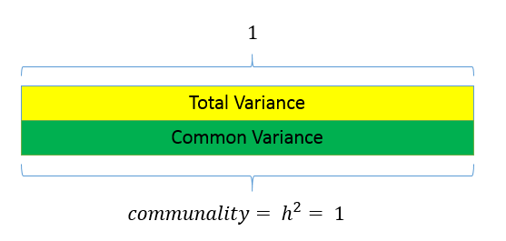
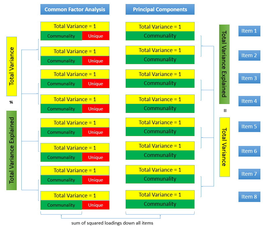
The figure below shows how these concepts are related:
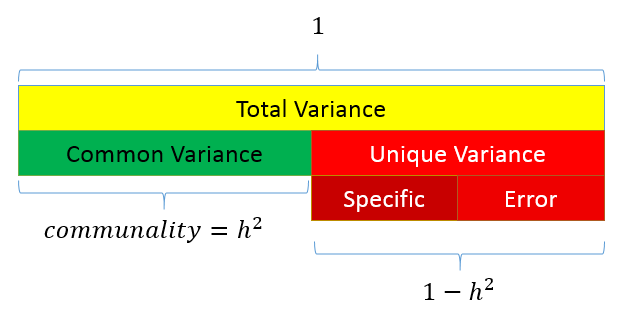 The total variance is made up to common variance and unique variance, and unique variance is composed of specific and error variance. If the total variance is 1, then the communality is \(h^2\) and the unique variance is \(1-h^2\). Let’s take a look at how the partition of variance applies to the SAQ-8 factor model.
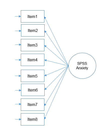
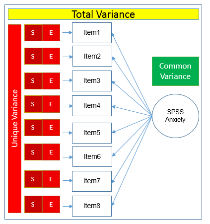 Here you see that SPSS Anxiety makes up the common variance for all eight items, but within each item there is specific variance and error variance. Take the example of Item 7 “Computers are useful only for playing games”. Although SPSS Anxiety explain some of this variance, there may be systematic factors such as technophobia and non-systemic factors that can’t be explained by either SPSS anxiety or technophbia, such as getting a speeding ticket right before coming to the survey center (error of meaurement). Now that we understand partitioning of variance we can move on to performing our first factor analysis. In fact, the assumptions we make about variance partitioning affects which analysis we run.
Performing Factor Analysis
As a data analyst, the goal of a factor analysis is to reduce the number of variables to explain and to interpret the results. This can be accomplished in two steps:
- factor extraction
- factor rotation
Factor extraction involves making a choice about the type of model as well the number of factors to extract. Factor rotation comes after the factors are extracted, with the goal of achieving simple structure in order to improve interpretability.
Extracting Factors
There are two approaches to factor extraction which stems from different approaches to variance partitioning: a) principal components analysis and b) common factor analysis.
Principal Components Analysis
Unlike factor analysis, principal components analysis or PCA makes the assumption that there is no unique variance, the total variance is equal to common variance. Recall that variance can be partitioned into common and unique variance. If there is no unique variance then common variance takes up total variance (see figure below). Additionally, if the total variance is 1, then the common variance is equal to the communality.
Running a PCA with 8 components in SPSS
The goal of a PCA is to replicate the correlation matrix using a set of components that are fewer in number and linear combinations of the original set of items. Although the following analysis defeats the purpose of doing a PCA we will begin by extracting as many components as possible as a teaching exercise and so that we can decide on the optimal number of components to extract later.
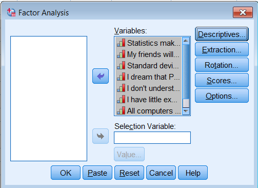
First go to Analyze – Dimension Reduction – Factor. Move all the observed variables over the Variables: box to be analyze.
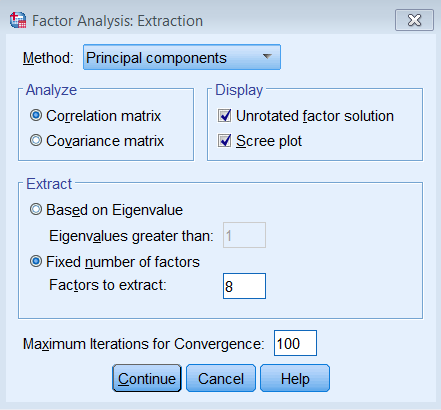
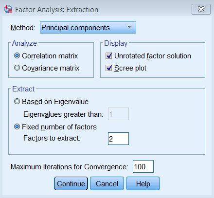
Under Extraction – Method, pick Principal components and make sure to Analyze the Correlation matrix. We also request the Unrotated factor solution and the Scree plot. Under Extract, choose Fixed number of factors, and under Factor to extract enter 8. We also bumped up the Maximum Iterations of Convergence to 100.
The equivalent SPSS syntax is shown below:
FACTOR
 /VARIABLES q01 q02 q03 q04 q05 q06 q07 q08
 /MISSING LISTWISE
 /ANALYSIS q01 q02 q03 q04 q05 q06 q07 q08
 /PRINT INITIAL EXTRACTION
 /PLOT EIGEN
 /CRITERIA FACTORS(8) ITERATE(100)
 /EXTRACTION PC
 /ROTATION NOROTATE
 /METHOD=CORRELATION.
Eigenvalues and Eigenvectors
Before we get into the SPSS output, let’s understand a few things about eigenvalues and eigenvectors.
Eigenvalues represent the total amount of variance that can be explained by a given principal component. They can be positive or negative in theory, but in practice they explain variance which is always positive.
- If eigenvalues are greater than zero, then it’s a good sign.
- Since variance cannot be negative, negative eigenvalues imply the model is ill-conditioned.
- Eigenvalues close to zero imply there is item multicollinearity, since all the variance can be taken up by the first component.
Eigenvalues are also the sum of squared component loadings across all items for each component, which represent the amount of variance in each item that can be explained by the principal component.
Eigenvectors represent a weight for each eigenvalue. The eigenvector times the square root of the eigenvalue gives the component loadings which can be interpreted as the correlation of each item with the principal component. For this particular PCA of the SAQ-8, the eigenvector associated with Item 1 on the first component is \(0.377\), and the eigenvalue of Item 1 is \(3.057\). We can calculate the first component as
$$(0.377)\sqrt{3.057}= 0.659.$$
In this case, we can say that the correlation of the first item with the first component is \(0.659\). Let’s now move on to the component matrix.
Component Matrix of the 8-component PCA
The components can be interpreted as the correlation of each item with the component. Each item has a loading corresponding to each of the 8 components. For example, Item 1 is correlated \(0.659\) with the first component, \(0.136\) with the second component and \(-0.398\) with the third, and so on.
The square of each loading represents the proportion of variance (think of it as an \(R^2\) statistic) explained by a particular component. For Item 1, \((0.659)^2=0.434\) or \(43.4\%\) of its variance is explained by the first component. Subsequently, \((0.136)^2 = 0.018\) or \(1.8\%\) of the variance in Item 1 is explained by the second component. The total variance explained by both components is thus \(43.4\%+1.8\%=45.2\%\). If you keep going on adding the squared loadings cumulatively down the components, you find that it sums to 1 or 100%. This is also known as the communality, and in a PCA the communality for each item is equal to the total variance.
| Component | ||||||||
| 1 | 2 | 3 | 4 | 5 | 6 | 7 | 8 | |
| Statistics makes me cry | .659 | .136 | -.398 | .160 | -.064 | .568 | -.177 | .068 |
| My friends will think I’m stupid for not being able to cope with SPSS | -.300 | .866 | -.025 | .092 | -.290 | -.170 | -.193 | -.001 |
| Standard deviations excite me | -.653 | .409 | .081 | .064 | .410 | .254 | .378 | .142 |
| I dream that Pearson is attacking me with correlation coefficients | .720 | .119 | -.192 | .064 | -.288 | -.089 | .563 | -.137 |
| I don’t understand statistics | .650 | .096 | -.215 | .460 | .443 | -.326 | -.092 | -.010 |
| I have little experience of computers | .572 | .185 | .675 | .031 | .107 | .176 | -.058 | -.369 |
| All computers hate me | .718 | .044 | .453 | -.006 | -.090 | -.051 | .025 | .516 |
| I have never been good at mathematics | .568 | .267 | -.221 | -.694 | .258 | -.084 | -.043 | -.012 |
| Extraction Method: Principal Component Analysis. | ||||||||
| a. 8 components extracted. | ||||||||
Summing the squared component loadings across the components (columns) gives you the communality estimates for each item, and summing each squared loading down the items (rows) gives you the eigenvalue for each component. For example, to obtain the first eigenvalue we calculate:
$$(0.659)^2 + (-.300)^2 + (-0.653)^2 + (0.720)^2 + (0.650)^2 + (0.572)^2 + (0.718)^2 + (0.568)^2 = 3.057$$
You will get eight eigenvalues for eight components, which leads us to the next table.
Total Variance Explained in the 8-component PCA
Recall that the eigenvalue represents the total amount of variance that can be explained by a given principal component. Starting from the first component, each subsequent component is obtained from partialling out the previous component. Therefore the first component explains the most variance, and the last component explains the least. Looking at the Total Variance Explained table, you will get the total variance explained by each component. For example, Component 1 is \(3.057\), or \((3.057/8)\% = 38.21\%\) of the total variance. Because we extracted the same number of components as the number of items, the Initial Eigenvalues column is the same as the Extraction Sums of Squared Loadings column.
| Component | Initial Eigenvalues | Extraction Sums of Squared Loadings | ||||
| Total | % of Variance | Cumulative % | Total | % of Variance | Cumulative % | |
| 1 | 3.057 | 38.206 | 38.206 | 3.057 | 38.206 | 38.206 |
| 2 | 1.067 | 13.336 | 51.543 | 1.067 | 13.336 | 51.543 |
| 3 | .958 | 11.980 | 63.523 | .958 | 11.980 | 63.523 |
| 4 | .736 | 9.205 | 72.728 | .736 | 9.205 | 72.728 |
| 5 | .622 | 7.770 | 80.498 | .622 | 7.770 | 80.498 |
| 6 | .571 | 7.135 | 87.632 | .571 | 7.135 | 87.632 |
| 7 | .543 | 6.788 | 94.420 | .543 | 6.788 | 94.420 |
| 8 | .446 | 5.580 | 100.000 | .446 | 5.580 | 100.000 |
| Extraction Method: Principal Component Analysis. | ||||||
Choosing the number of components to extract
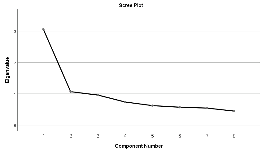
Since the goal of running a PCA is to reduce our set of variables down, it would useful to have a criterion for selecting the optimal number of components that are of course smaller than the total number of items. One criterion is the choose components that have eigenvalues greater than 1. Under the Total Variance Explained table, we see the first two components have an eigenvalue greater than 1. This can be confirmed by the Scree Plot which plots the eigenvalue (total variance explained) by the component number. Recall that we checked the Scree Plot option under Extraction – Display, so the scree plot should be produced automatically.
The first component will always have the highest total variance and the last component will always have the least, but where do we see the largest drop? If you look at Component 2, you will see an “elbow” joint. This is the marking point where it’s perhaps not too beneficial to continue further component extraction. Using the scree plot we pick two components.
Some criteria say that the total variance explained by all components should be between 70% to 80% variance, which in this case would mean about four to five components. The authors of the book say that this may be untenable for social science research where extracted factors usually explain only 50% to 60%. Picking the number of components is a bit of an art and requires input from the whole research team. Let’s suppose we talked to the principal investigator and she believes that the two component solution makes sense for the study, so we will proceed with the analysis.
Running a PCA with 2 components in SPSS
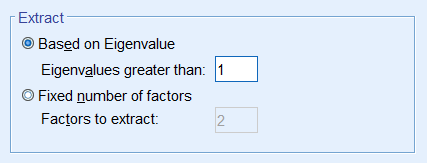
Running the two component PCA is just as easy as running the 8 component solution. The only difference is under Fixed number of factors – Factors to extract you enter 2.
We will focus the differences in the output between the eight and two-component solution. Under Total Variance Explained, we see that the Initial Eigenvalues no longer equals the Extraction Sums of Squared Loadings. The main difference is that there are only two rows of eigenvalues, and the cumulative percent variance goes up to \(51.54\%\).
| Component | Initial Eigenvalues | Extraction Sums of Squared Loadings | ||||
| Total | % of Variance | Cumulative % | Total | % of Variance | Cumulative % | |
| 1 | 3.057 | 38.206 | 38.206 | 3.057 | 38.206 | 38.206 |
| 2 | 1.067 | 13.336 | 51.543 | 1.067 | 13.336 | 51.543 |
| 3 | .958 | 11.980 | 63.523 | |||
| 4 | .736 | 9.205 | 72.728 | |||
| 5 | .622 | 7.770 | 80.498 | |||
| 6 | .571 | 7.135 | 87.632 | |||
| 7 | .543 | 6.788 | 94.420 | |||
| 8 | .446 | 5.580 | 100.000 | |||
| Extraction Method: Principal Component Analysis. | ||||||
Again, we interpret Item 1 as having a correlation of 0.659 with Component 1. From glancing at the solution, we see that Item 4 has the highest correlation with Component 1 and Item 2 the lowest. Similarly, we see that Item 2 has the highest correlation with Component 2 and Item 7 the lowest.
Quick check:
True or False
- The elements of the Component Matrix are correlations of the item with each component.
- The sum of the squared eigenvalues is the proportion of variance under Total Variance Explained.
- The Component Matrix can be thought of as correlations and the Total Variance Explained table can be thought of as \(R^2\).
1.T, 2.F (sum of squared loadings), 3. T
Communalities of the 2-component PCA
The communality is the sum of the squared component loadings up to the number of components you extract. In the SPSS output you will see a table of communalities.
| Initial | Extraction | |
| Statistics makes me cry | 1.000 | .453 |
| My friends will think I’m stupid for not being able to cope with SPSS | 1.000 | .840 |
| Standard deviations excite me | 1.000 | .594 |
| I dream that Pearson is attacking me with correlation coefficients | 1.000 | .532 |
| I don’t understand statistics | 1.000 | .431 |
| I have little experience of computers | 1.000 | .361 |
| All computers hate me | 1.000 | .517 |
| I have never been good at mathematics | 1.000 | .394 |
| Extraction Method: Principal Component Analysis. | ||
Since PCA is an iterative estimation process, it starts with 1 as an initial estimate of the communality (since this is the total variance across all 8 components), and then proceeds with the analysis until a final communality extracted. Notice that the Extraction column is smaller than the Initial column because we only extracted two components. As an exercise, let’s manually calculate the first communality from the Component Matrix. The first ordered pair is \((0.659,0.136)\) which represents the correlation of the first item with Component 1 and Component 2. Recall that squaring the loadings and summing down the components (columns) gives us the communality:
$$h^2_1 = (0.659)^2 + (0.136)^2 = 0.453$$
Going back to the Communalities table, if you sum down all 8 items (rows) of the Extraction column, you get \(4.123\). If you go back to the Total Variance Explained table and summed the first two eigenvalues you also get \(3.057+1.067=4.124\). Is that surprising? Basically it’s saying that the summing the communalities across all items is the same as summing the eigenvalues across all components.
Quiz
1. In an 8-component PCA, how many components must you extract so that the communality for the Initial column is equal to the Extraction column?
Answer: 8
True or False
- The eigenvalue represents the communality for each item.
- For a single component, the sum of squared component loadings across all items represents the eigenvalue for that component.
- The sum of eigenvalues for all the components is the total variance.
- The sum of the communalities down the components is equal to the sum of eigenvalues down the items.
Answers:
1. F, the eigenvalue is the total communality across all items for a single component, 2. T, 3. T, 4. F (you can only sum communalities across items, and sum eigenvalues across components, but if you do that they are equal).
Common Factor Analysis
The partitioning of variance differentiates a principal components analysis from what we call common factor analysis. Both methods try to reduce the dimensionality of the dataset down to fewer unobserved variables, but whereas PCA assumes that there common variances takes up all of total variance, common factor analysis assumes that total variance can be partitioned into common and unique variance. It is usually more reasonable to assume that you have not measured your set of items perfectly. The unobserved or latent variable that makes up common variance is called a factor, hence the name factor analysis. The other main difference between PCA and factor analysis lies in the goal of your analysis. If your goal is to simply reduce your variable list down into a linear combination of smaller components then PCA is the way to go. However, if you believe there is some latent construct that defines the interrelationship among items, then factor analysis may be more appropriate. In this case, we assume that there is a construct called SPSS Anxiety that explains why you see a correlation among all the items on the SAQ-8, we acknowledge however that SPSS Anxiety cannot explain all the shared variance among items in the SAQ, so we model the unique variance as well. Based on the results of the PCA, we will start with a two factor extraction.
Running a Common Factor Analysis with 2 factors in SPSS
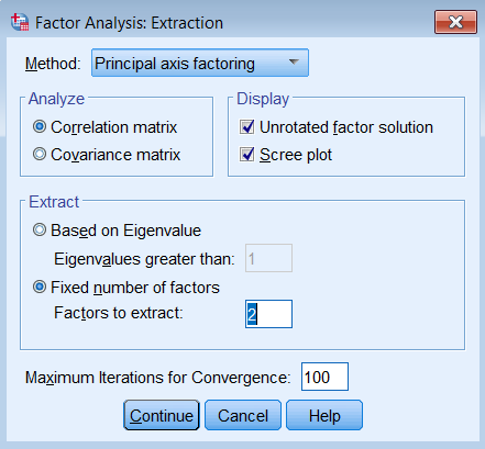
To run a factor analysis, use the same steps as running a PCA (Analyze – Dimension Reduction – Factor) except under Method choose Principal axis factoring. Note that we continue to set Maximum Iterations for Convergence at 100 and we will see why later.
Pasting the syntax into the SPSS Syntax Editor we get:
FACTOR
 /VARIABLES q01 q02 q03 q04 q05 q06 q07 q08
 /MISSING LISTWISE
 /ANALYSIS q01 q02 q03 q04 q05 q06 q07 q08
 /PRINT INITIAL EXTRACTION
 /PLOT EIGEN
 /CRITERIA FACTORS(2) ITERATE(100)
 /EXTRACTION PAF
 /ROTATION NOROTATE
 /METHOD=CORRELATION.
Note the main difference is under /EXTRACTION we list PAF for Principal Axis Factoring instead of PC for Principal Components. We will get three tables of output, Communalities, Total Variance Explained and Factor Matrix. Let’s go over each of these and compare them to the PCA output.
Communalities of the 2-factor PAF
| Initial | Extraction | |
| Statistics makes me cry | .293 | .437 |
| My friends will think I’m stupid for not being able to cope with SPSS | .106 | .052 |
| Standard deviations excite me | .298 | .319 |
| I dream that Pearson is attacking me with correlation coefficients | .344 | .460 |
| I don’t understand statistics | .263 | .344 |
| I have little experience of computers | .277 | .309 |
| All computers hate me | .393 | .851 |
| I have never been good at mathematics | .192 | .236 |
| Extraction Method: Principal Axis Factoring. | ||
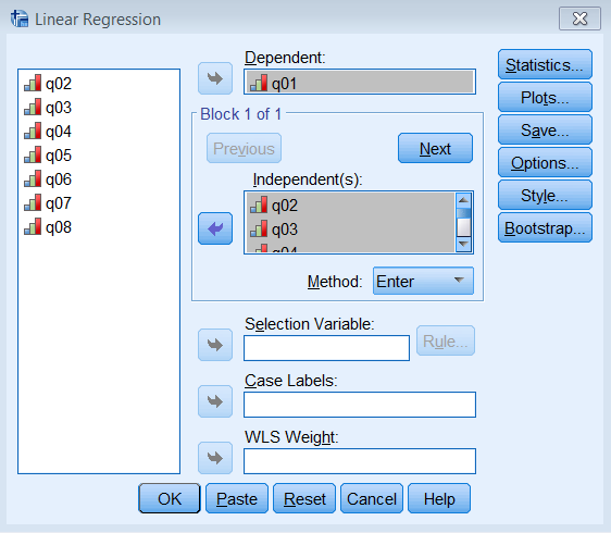
The most striking difference between this communalities table and the one from the PCA is that the initial extraction is no longer one. Recall that for a PCA, we assume the total variance is completely taken up by the common variance or communality, and therefore we pick 1 as our best initial guess. What principal axis factoring does is instead of guessing 1 as the initial communality, it chooses the squared multiple correlation coefficient \(R^2\). To see this in action for Item 1 run a linear regression where Item 1 is the dependent variable and Items 2 -8 are independent variables. Go to Analyze – Regression – Linear and enter q01 under Dependent and q02 to q08 under Independent(s).
Pasting the syntax into the Syntax Editor gives us:
REGRESSION
 /MISSING LISTWISE
 /STATISTICS COEFF OUTS R ANOVA
 /CRITERIA=PIN(.05) POUT(.10)
 /NOORIGIN
 /DEPENDENT q01
 /METHOD=ENTER q02 q03 q04 q05 q06 q07 q08.
The output we obtain from this analysis is
| Model | R | R Square | Adjusted R Square | Std. Error of the Estimate |
| 1 | .541a | .293 | .291 | .697 |
| a. Predictors: (Constant), I have never been good at mathematics, My friends will think I’m stupid for not being able to cope with SPSS, I have little experience of computers, I don’t understand statistics, Standard deviations excite me, I dream that Pearson is attacking me with correlation coefficients, All computers hate me | ||||
Note that 0.293 (bolded) matches the initial communality estimate for Item 1. We can do eight more linear regressions in order to get all eight communality estimates but SPSS already does that for us. Like PCA, factor analysis also uses an iterative estimation process to obtain the final estimates under the Extraction column. Finally, summing all the rows of the extraction column, and we get 3.00. This represents the total common variance shared among all items for a two factor solution.
Total Variance Explained (2-factor PAF)
The next table we will look at is Total Variance Explained. Comparing this to the table from the PCA we notice that the Initial Eigenvalues are exactly the same and includes 8 rows for each “factor”. In fact, SPSS simply borrows the information from the PCA analysis for use in the factor analysis and the factors are actually components in the Initial Eigenvalues column. The main difference now is in the Extraction Sums of Squares Loadings. We notice that each corresponding row in the Extraction column is lower than the Initial column. This is expected because we assume that total variance can be partitioned into common and unique variance, which means the common variance explained will be lower. Factor 1 explains 31.38% of the variance whereas Factor 2 explains 6.24% of the variance. Just as in PCA the more factors you extract, the less variance explained by each successive factor.
| Factor | Initial Eigenvalues | Extraction Sums of Squared Loadings | ||||
| Total | % of Variance | Cumulative % | Total | % of Variance | Cumulative % | |
| 1 | 3.057 | 38.206 | 38.206 | 2.511 | 31.382 | 31.382 |
| 2 | 1.067 | 13.336 | 51.543 | .499 | 6.238 | 37.621 |
| 3 | .958 | 11.980 | 63.523 | |||
| 4 | .736 | 9.205 | 72.728 | |||
| 5 | .622 | 7.770 | 80.498 | |||
| 6 | .571 | 7.135 | 87.632 | |||
| 7 | .543 | 6.788 | 94.420 | |||
| 8 | .446 | 5.580 | 100.000 | |||
| Extraction Method: Principal Axis Factoring. | ||||||
A subtle note that may be easily overlooked is that when SPSS plots the scree plot or the Eigenvalues greater than 1 criterion (Analyze – Dimension Reduction – Factor – Extraction), it bases it off the Initial and not the Extraction solution. This is important because the criterion here assumes no unique variance as in PCA, which means that this is the total variance explained not accounting for specific or measurement error. Note that in the Extraction of Sums Squared Loadings column the second factor has an eigenvalue that is less than 1 but is still retained because the Initial value is 1.067. If you want to use this criterion for the common variance explained you would need to modify the criterion yourself.
Quick Quiz
- In theory, when would the percent of variance in the Initial column ever equal the Extraction column?
- True or False, in SPSS when you use the Principal Axis Factor method the scree plot uses the final factor analysis solution to plot the eigenvalues.
Answers: 1. When there is no unique variance (PCA assumes this whereas common factor analysis does not, so this is in theory and not in practice), 2. F, it uses the initial PCA solution and the eigenvalues assume no unique variance.
Factor Matrix (2-factor PAF)
| Factor | ||
| 1 | 2 | |
| Statistics makes me cry | .588 | -.303 |
| My friends will think I’m stupid for not being able to cope with SPSS | -.227 | .020 |
| Standard deviations excite me | -.557 | .094 |
| I dream that Pearson is attacking me with correlation coefficients | .652 | -.189 |
| I don’t understand statistics | .560 | -.174 |
| I have little experience of computers | .498 | .247 |
| All computers hate me | .771 | .506 |
| I have never been good at mathematics | .470 | -.124 |
| Extraction Method: Principal Axis Factoring. | ||
| a. 2 factors extracted. 79 iterations required. | ||
First note the annotation that 79 iterations were required. If we had simply used the default 25 iterations in SPSS, we would not have obtained an optimal solution. This is why in practice it’s always good to increase the maximum number of iterations. Now let’s get into the table itself. The elements of the Factor Matrix table are called loadings and represent the correlation of each item with the corresponding factor. Just as in PCA, squaring each loading and summing down the items (rows) gives the total variance explained by each factor. Note that they are no longer called eigenvalues as in PCA. Let’s calculate this for Factor 1:
$$(0.588)^2 + (-0.227)^2 + (-0.557)^2 + (0.652)^2 + (0.560)^2 + (0.498)^2 + (0.771)^2 + (0.470)^2 = 2.51$$
This number matches the first row under the Extraction column of the Total Variance Explained table. We can repeat this for Factor 2 and get matching results for the second row. Additionally, we can get the communality estimates by summing the squared loadings across the factors (columns) for each item. For example, for Item 1:
$$(0.588)^2 + (-0.303)^2 = 0.437$$
Note that these results match the value of the Communalities table for Item 1 under the Extraction column. This means that the sum of squared loadings across factors represents the communality estimates for each item.
Practical Interpretation
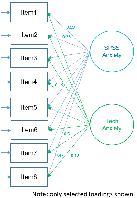
The figure below shows the path diagram of the orthogonal two-factor EFA solution show above (note that only selected loadings are shown). The loadings represent zero-order correlations of a particular factor with each item. Looking at absolute loadings greater than 0.4, Items 1,3,4,5 and 7 loading strongly onto Factor 1 and only Item 4 (e.g., “All computers hate me”) loads strongly onto Factor 2. From speaking with the Principal Investigator, we hypothesize that the second factor corresponds to general anxiety with technology rather than anxiety in particular to SPSS. However, use caution when interpretation unrotated solutions, as these represent loadings where the first factor explains maximum variance (notice that most high loadings are concentrated in first factor). In the sections below, we will see how factor rotations can change the interpretation of these loadings.
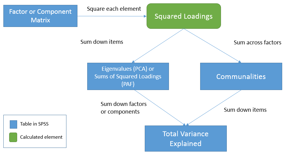
The relationship between the three tables
To see the relationships among the three tables let’s first start from the Factor Matrix (or Component Matrix in PCA). We will use the term factor to represent components in PCA as well. These elements represent the correlation of the item with each factor. Now, square each element to obtain squared loadings or the proportion of variance explained by each factor for each item. Summing the squared loadings across factors you get the proportion of variance explained by all factors in the model. This is known as common variance or communality, hence the result is the Communalities table. Going back to the Factor Matrix, if you square the loadings and sum down the items you get Sums of Squared Loadings (in PAF) or eigenvalues (in PCA) for each factor. These now become elements of the Total Variance Explained table. Summing down the rows (i.e., summing down the factors) under the Extraction column we get \(2.511 + 0.499 = 3.01\) or the total (common) variance explained. In words, this is the total (common) variance explained by the two factor solution for all eight items. Equivalently, since the Communalities table represents the total common variance explained by both factors for each item, summing down the items in the Communalities table also gives you the total (common) variance explained, in this case
$$ (0.437)^2 + (0.052)^2 + (0.319)^2 + (0.460)^2 + (0.344)^2 + (0.309)^2 + (0.851)^2 + (0.236)^2 = 3.01$$
which is the same result we obtained from the Total Variance Explained table. Here is a table that that may help clarify what we’ve talked about:
In summary:
- Squaring the elements in the Component Matrix or Factor Matrix gives you the squared loadings
- Summing the squared loadings of the Factor Matrix across the factors gives you the communality estimates for each item in the Extraction column of the Communalities table.
- Summing the squared loadings of the Factor Matrix down the items gives you the Sums of Squared Loadings (PAF) or eigenvalue (PCA) for each factor across all items.
- Summing the eigenvalues (PCA) or Sums of Squared Loadings (PAF) in the Total Variance Explained table gives you the total common variance explained.
- Summing down all items of the Communalities table is the same as summing the eigenvalues (PCA) or Sums of Squared Loadings (PCA) down all components or factors under the Extraction column of the Total Variance Explained table.
Quiz
True or False (the following assumes a two-factor Principal Axis Factor solution with 8 items)
- The elements of the Factor Matrix represent correlations of each item with a factor.
- Each squared element of Item 1 in the Factor Matrix represents the communality.
- Summing the squared elements of the Factor Matrix down all 8 items within Factor 1 equals the first Sums of Squared Loadings under the Extraction column of Total Variance Explained table.
- Summing down all 8 items in the Extraction column of the Communalities table gives us the total common variance explained by both factors.
- The total common variance explained is obtained by summing all Sums of Squared Loadings of the Initial column of the Total Variance Explained table
- The total Sums of Squared Loadings in the Extraction column under the Total Variance Explained table represents the total variance which consists of total common variance plus unique variance.
- In common factor analysis, the Sums of Squared loadings is the eigenvalue.
Answers: 1. T, 2. F, the sum of the squared elements across both factors, 3. T, 4. T, 5. F, sum all Sums of Squared Loadings from the Extraction column of the Total Variance Explained table, 6. F, the total Sums of Squared Loadings represents only the total common variance excluding unique variance, 7. F, eigenvalues are only applicable for PCA.
Maximum Likelihood Estimation (2-factor ML)
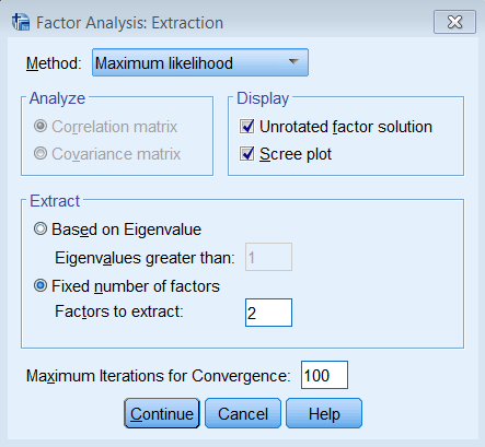
Since this is a non-technical introduction to factor analysis, we won’t go into detail about the differences between Principal Axis Factoring (PAF) and Maximum Likelihood (ML). The main concept to know is that ML also assumes a common factor analysis using the \(R^2\) to obtain initial estimates of the communalities, but uses a different iterative process to obtain the extraction solution. To run a factor analysis using maximum likelihood estimation under Analyze – Dimension Reduction – Factor – Extraction – Method choose Maximum Likelihood.
Although the initial communalities are the same between PAF and ML, the final extraction loadings will be different, which means you will have different Communalities, Total Variance Explained, and Factor Matrix tables (although Initial columns will overlap). The other main difference is that you will obtain a Goodness-of-fit Test table, which gives you a absolute test of model fit. Non-significant values suggest a good fitting model. Here the p-value is less than 0.05 so we reject the two-factor model.
| Chi-Square | df | Sig. |
| 198.617 | 13 | .000 |
In practice, you would obtain chi-square values for multiple factor analysis runs, which we tabulate below from 1 to 8 factors. The table shows the number of factors extracted (or attempted to extract) as well as the chi-square, degrees of freedom, p-value and iterations needed to converge. Note that as you increase the number of factors, the chi-square value and degrees of freedom decreases but the iterations needed and p-value increases. Practically, you want to make sure the number of iterations you specify exceeds the iterations needed. Additionally, NS means no solution and N/A means not applicable. In SPSS, no solution is obtained when you run 5 to 7 factors because the degrees of freedom is negative (which cannot happen). For the eight factor solution, it is not even applicable in SPSS because it will spew out a warning that “You cannot request as many factors as variables with any extraction method except PC. The number of factors will be reduced by one.” This means that if you try to extract an eight factor solution for the SAQ-8, it will default back to the 7 factor solution. Now that we understand the table, let’s see if we can find the threshold at which the absolute fit indicates a good fitting model. It looks like here that the p-value becomes non-significant at a 3 factor solution. Note that differs from the eigenvalues greater than 1 criterion which chose 2 factors and using Percent of Variance explained you would choose 4-5 factors. We talk to the Principal Investigator and at this point, we still prefer the two-factor solution. Note that there is no “right” answer in picking the best factor model, only what makes sense for your theory. We will talk about interpreting the factor loadings when we talk about factor rotation to further guide us in choosing the correct number of factors.
| Number of Factors | Chi-square | Df | p-value | Iterations needed |
| 1 | 553.08 | 20 | <0.05 | 4 |
| 2 | 198.62 | 13 | < 0.05 | 39 |
| 3 | 13.81 | 7 | 0.055 | 57 |
| 4 | 1.386 | 2 | 0.5 | 168 |
| 5 | NS | -2 | NS | NS |
| 6 | NS | -5 | NS | NS |
| 7 | NS | -7 | NS | NS |
| 8 | N/A | N/A | N/A | N/A |
Quiz
True or False
- The Initial column of the Communalities table for the Principal Axis Factoring and the Maximum Likelihood method are the same given the same analysis.
- Since they are both factor analysis methods, Principal Axis Factoring and the Maximum Likelihood method will result in the same Factor Matrix.
- In SPSS, both Principal Axis Factoring and Maximum Likelihood methods give chi-square goodness of fit tests.
- You can extract as many factors as there are items as when using ML or PAF.
- When looking at the Goodness-of-fit Test table, a p-value less than 0.05 means the model is a good fitting model.
- In the Goodness-of-fit Test table, the lower the degrees of freedom the more factors you are fitting.
Answers: 1. T, 2. F, the two use the same starting communalities but a different estimation process to obtain extraction loadings, 3. F, only Maximum Likelihood gives you chi-square values, 4. F, you can extract as many components as items in PCA, but SPSS will only extract up to the total number of items minus 1, 5. F, greater than 0.05, 6. T, we are taking away degrees of freedom but extracting more factors.
Comparing Common Factor Analysis versus Principal Components
As we mentioned before, the main difference between common factor analysis and principal components is that factor analysis assumes total variance can be partitioned into common and unique variance, whereas principal components assumes common variance takes up all of total variance (i.e., no unique variance). For both methods, when you assume total variance is 1, the common variance becomes the communality. The communality is unique to each item, so if you have 8 items, you will obtain 8 communalities; and it represents the common variance explained by the factors or components. However in the case of principal components, the communality is the total variance of each item, and summing all 8 communalities gives you the total variance across all items. In contrast, common factor analysis assumes that the communality is a portion of the total variance, so that summing up the communalities represents the total common variance and not the total variance. In summary, for PCA, total common variance is equal to total variance explained, which in turn is equal to the total variance, but in common factor analysis, total common variance is equal to total variance explained but does not equal total variance.
Quiz
True or False
The following applies to the SAQ-8 when theoretically extracting 8 components or factors for 8 items:
- Theoretically, if there is no unique variance the communality would equal total variance.
- In principal components, each communality represents the total variance across all 8 items.
- In common factor analysis, the communality represents the common variance for each item.
- The communality is unique to each factor or component.
- For both PCA and common factor analysis, the sum of the communalities represent the total variance explained.
- For PCA, the total variance explained equals the total variance, but for common factor analysis it does not.
Answers: 1. T, 2. F, the total variance for each item, 3. T, 4. F, communality is unique to each item (shared across components or factors), 5. T, 6. T.
Rotation Methods
After deciding on the number of factors to extract and with analysis model to use, the next step is to interpret the factor loadings. Factor rotations help us interpret factor loadings. There are two general types of rotations, orthogonal and oblique.
- orthogonal rotation assume factors are independent or uncorrelated with each other
- oblique rotation factors are not independent and are correlated
The goal of factor rotation is to improve the interpretability of the factor solution by reaching simple structure.
Simple structure
Without rotation, the first factor is the most general factor onto which most items load and explains the largest amount of variance. This may not be desired in all cases. Suppose you wanted to know how well a set of items load on each factor; simple structure helps us to achieve this.
The definition of simple structure is that in a factor loading matrix:
- Each row should contain at least one zero.
- For m factors, each column should have at least m zeroes (e.g., three factors, at least 3 zeroes per factor).
For every pair of factors (columns),
- there should be several items for which entries approach zero in one column but large loadings on the other.
- a large proportion of items should have entries approaching zero.
- only a small number of items have two non-zero entries.
The following table is an example of simple structure with three factors:
| Item | Factor 1 | Factor 2 | Factor 3 |
| 1 | 0.8 | 0 | 0 |
| 2 | 0.8 | 0 | 0 |
| 3 | 0.8 | 0 | 0 |
| 4 | 0 | 0.8 | 0 |
| 5 | 0 | 0.8 | 0 |
| 6 | 0 | 0.8 | 0 |
| 7 | 0 | 0 | 0.8 |
| 8 | 0 | 0 | 0.8 |
Let’s go down the checklist of criteria to see why it satisfies simple structure:
- each row contains at least one zero (exactly two in each row)
- each column contains at least three zeros (since there are three factors)
- for every pair of factors, most items have zero on one factor and non-zeros on the other factor (e.g., looking at Factors 1 and 2, Items 1 through 6 satisfy this requirement)
- for every pair of factors, all items have zero entries
- for every pair of factors, none of the items have two non-zero entries
An easier set of criteria from Pedhazur and Schemlkin (1991) states that
- each item has high loadings on one factor only
- each factor has high loadings for only some of the items.
Quiz
For the following factor matrix, explain why it does not conform to simple structure using both the conventional and Pedhazur test.
| Item | Factor 1 | Factor 2 | Factor 3 |
| 1 | 0.8 | 0 | 0.8 |
| 2 | 0.8 | 0 | 0.8 |
| 3 | 0.8 | 0 | 0 |
| 4 | 0.8 | 0 | 0 |
| 5 | 0 | 0.8 | 0.8 |
| 6 | 0 | 0.8 | 0.8 |
| 7 | 0 | 0.8 | 0.8 |
| 8 | 0 | 0.8 | 0 |
Solution: Using the conventional test, although Criteria 1 and 2 are satisfied (each row has at least one zero, each column has at least three zeroes), Criterion 3 fails because for Factors 2 and 3, only 3/8 rows have 0 on one factor and non-zero on the other. Additionally, for Factors 2 and 3, only Items 5 through 7 have non-zero loadings or 3/8 rows have non-zero coefficients (fails Criteria 4 and 5 simultaneously). Using the Pedhazur method, Items 1, 2, 5, 6, and 7 have high loadings on two factors (fails first criterion) and Factor 3 has high loadings on a majority or 5 out of 8 items (fails second criterion).
Orthogonal Rotation (2 factor PAF)
We know that the goal of factor rotation is to rotate the factor matrix so that it can approach simple structure in order to improve interpretability. Orthogonal rotation assumes that the factors are not correlated. The benefit of doing an orthogonal rotation is that loadings are simple correlations of items with factors, and standardized solutions can estimate the unique contribution of each factor. The most common type of orthogonal rotation is Varimax rotation. We will walk through how to do this in SPSS.
Running a two-factor solution (PAF) with Varimax rotation in SPSS
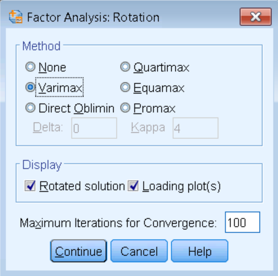
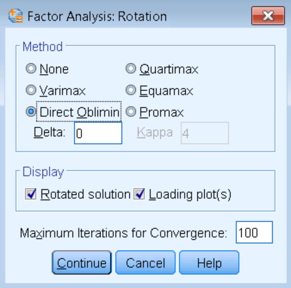
The steps to running a two-factor Principal Axis Factoring is the same as before (Analyze – Dimension Reduction – Factor – Extraction), except that under Rotation – Method we check Varimax. Make sure under Display to check Rotated Solution and Loading plot(s), and under Maximum Iterations for Convergence enter 100.
Pasting the syntax into the SPSS editor you obtain:
FACTOR
 /VARIABLES q01 q02 q03 q04 q05 q06 q07 q08
 /MISSING LISTWISE
 /ANALYSIS q01 q02 q03 q04 q05 q06 q07 q08
 /PRINT INITIAL EXTRACTION ROTATION
 /PLOT ROTATION
 /CRITERIA FACTORS(2) ITERATE(100)
 /EXTRACTION PAF
 /CRITERIA ITERATE(100)
 /ROTATION VARIMAX
 /METHOD=CORRELATION.
Let’s first talk about what tables are the same or different from running a PAF with no rotation. First, we know that the unrotated factor matrix (Factor Matrix table) should be the same. Additionally, since the common variance explained by both factors should be the same, the Communalities table should be the same. The main difference is that we ran a rotation, so we should get the rotated solution (Rotated Factor Matrix) as well as the transformation used to obtain the rotation (Factor Transformation Matrix). Finally, although the total variance explained by all factors stays the same, the total variance explained by each factor will be different.
Rotated Factor Matrix (2-factor PAF Varimax)
| Factor | ||
| 1 | 2 | |
| Statistics makes me cry | .646 | .139 |
| My friends will think I’m stupid for not being able to cope with SPSS | -.188 | -.129 |
| Standard deviations excite me | -.490 | -.281 |
| I dream that Pearson is attacking me with correlation coefficients | .624 | .268 |
| I don’t understand statistics | .544 | .221 |
| I have little experience of computers | .229 | .507 |
| All computers hate me | .275 | .881 |
| I have never been good at mathematics | .442 | .202 |
| Extraction Method: Principal Axis Factoring. Rotation Method: Varimax with Kaiser Normalization. | ||
| a. Rotation converged in 3 iterations. | ||
The Rotated Factor Matrix table tells us what the factor loadings look like after rotation (in this case Varimax). Kaiser normalization is a method to obtain stability of solutions across samples. After rotation, the loadings are rescaled back to the proper size. This means that equal weight is given to all items when performing the rotation. The only drawback is if the communality is low for a particular item, Kaiser normalization will weight these items equally with items with high communality. As such, Kaiser normalization is preferred when communalities are high across all items. You can turn off Kaiser normalization by specifying
/CRITERIA NOKAISER
Here is what the Varimax rotated loadings look like without Kaiser normalization. Compared to the rotated factor matrix with Kaiser normalization the patterns look similar if you flip Factors 1 and 2; this may be an artifact of the rescaling. The biggest difference between the two solutions is for items with low communalities such as Item 2 (0.052) and Item 8 (0.236). Kaiser normalization weights these items equally with the other high communality items.
| Factor | ||
| 1 | 2 | |
| Statistics makes me cry | .207 | .628 |
| My friends will think I’m stupid for not being able to cope with SPSS | -.148 | -.173 |
| Standard deviations excite me | -.331 | -.458 |
| I dream that Pearson is attacking me with correlation coefficients | .332 | .592 |
| I don’t understand statistics | .277 | .517 |
| I have little experience of computers | .528 | .174 |
| All computers hate me | .905 | .180 |
| I have never been good at mathematics | .248 | .418 |
| Extraction Method: Principal Axis Factoring. Rotation Method: Varimax without Kaiser Normalization. | ||
| a. Rotation converged in 3 iterations. | ||
Interpreting the factor loadings (2-factor PAF Varimax)
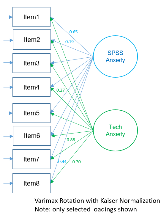
In the both the Kaiser normalized and non-Kaiser normalized rotated factor matrices, the loadings that have a magnitude greater than 0.4 are bolded. We can see that Items 6 and 7 load highly onto Factor 1 and Items 1, 3, 4, 5, and 8 load highly onto Factor 2. Item 2 does not seem to load highly on any factor. Looking more closely at Item 6 “My friends are better at statistics than me” and Item 7 “Computers are useful only for playing games”, we don’t see a clear construct that defines the two. Item 2, “I don’t understand statistics” may be too general an item and isn’t captured by SPSS Anxiety. The figure below shows the path diagram of the Varimax rotation. Comparing this solution to the unrotated solution, we notice that there are high loadings in both Factor 1 and 2. This is because Varimax maximizes the sum of the variances of the squared loadings, which in effect maximizes high loadings and minimizes low loadings.
Factor Transformation Matrix and Factor Loading Plot (2-factor PAF Varimax)
The Factor Transformation Matrix tells us how the Factor Matrix was rotated. In SPSS, you will see a matrix with two rows and two columns because we have two factors.
| Factor | 1 | 2 |
| 1 | .773 | .635 |
| 2 | -.635 | .773 |
| Extraction Method: Principal Axis Factoring. Rotation Method: Varimax with Kaiser Normalization. | ||
How do we interpret this matrix? Well, we can see it as the way to move from the Factor Matrix to the Kaiser-normalized Rotated Factor Matrix. From the Factor Matrix we know that the loading of Item 1 on Factor 1 is \(0.588\) and the loading of Item 1 on Factor 2 is \(-0.303\), which gives us the pair \((0.588,-0.303)\); but in the Kaiser-normalized Rotated Factor Matrix the new pair is \((0.646,0.139)\). How do we obtain this new transformed pair of values? We can do what’s called matrix multiplication. The steps are essentially to start with one column of the Factor Transformation matrix, view it as another ordered pair and multiply matching ordered pairs. To get the first element, we can multiply the ordered pair in the Factor Matrix \((0.588,-0.303)\) with the matching ordered pair \((0.773,-0.635)\) in the first column of the Factor Transformation Matrix.
$$(0.588)(0.773)+(-0.303)(-0.635)=0.455+0.192=0.647.$$
To get the second element, we can multiply the ordered pair in the Factor Matrix \((0.588,-0.303)\) with the matching ordered pair \((0.635, 0.773)\) from the second column of the Factor Transformation Matrix:
$$(0.588)(0.635)+(-0.303)(0.773)=0.373-0.234=0.139.$$
Voila! We have obtained the new transformed pair with some rounding error. The figure below summarizes the steps we used to perform the transformation
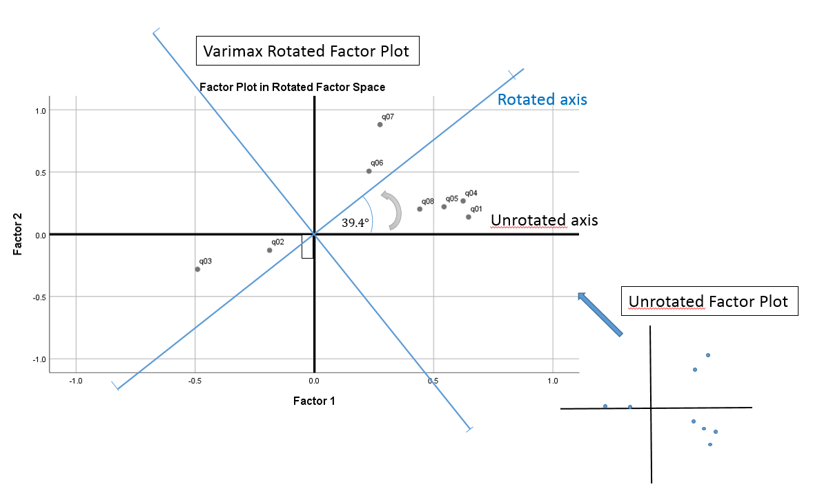
The Factor Transformation Matrix can also tell us angle of rotation if we take the inverse cosine of the diagonal element. In this case, the angle of rotation is \(cos^{-1}(0.773) =39.4 ^{\circ}\). In the factor loading plot, you can see what that angle of rotation looks like, starting from \(0^{\circ}\) rotating up in a counterclockwise direction by \(39.4^{\circ}\). Notice here that the newly rotated x and y-axis are still at \(90^{\circ}\) angles from one another, hence the name orthogonal (a non-orthogonal or oblique rotation means that the new axis is no longer \(90^{\circ}\) apart). Notice that the original loadings do not move with respect to the original axis, which means you are simply re-defining the axis for the same loadings.
Total Variance Explained (2-factor PAF Varimax)
The Total Variance Explained table contains the same columns as the PAF solution with no rotation, but adds another set of columns called “Rotation Sums of Squared Loadings”. This makes sense because if our rotated Factor Matrix is different, the square of the loadings should be different, and hence the Sum of Squared loadings will be different for each factor. However, if you sum the Sums of Squared Loadings across all factors for the Rotation solution,
$$ 1.521 + 1.489 = 3.01$$
and for the unrotated solution,
$$ 2.511 + 0.499 = 3.01,$$
you will see that the two sums are the same. This is because rotation does not change the total common variance. Looking at the Rotation Sums of Squared Loadings for Factor 1, it still has the largest total variance, but now that shared variance is split more evenly.
| Factor | Extraction Sums of Squared Loadings | Rotation Sums of Squared Loadings | ||||
| Total | % of Variance | Cumulative % | Total | % of Variance | Cumulative % | |
| 1 | 2.511 | 31.382 | 31.382 | 1.521 | 19.010 | 19.010 |
| 2 | .499 | 6.238 | 37.621 | 1.489 | 18.610 | 37.621 |
| Extraction Method: Principal Axis Factoring. | ||||||
Other Orthogonal Rotations
Varimax rotation is the most popular orthogonal rotation. The benefit of Varimax rotation is that it maximizes the variances of the loadings within the factors while maximizing differences between high and low loadings on a particular factor. Higher loadings are made higher while lower loadings are made lower. This makes Varimax rotation good for achieving simple structure but not as good for detecting an overall factor because it splits up variance of major factors among lesser ones. Quartimax may be a better choice for detecting an overall factor. It maximizes the squared loadings so that each item loads most strongly onto a single factor.
Here is the output of the Total Variance Explained table juxtaposed side-by-side for Varimax versus Quartimax rotation.
| Factor | Rotation Sums of Squared Loadings (Varimax) | Rotation Sums of Squared Loadings (Quartimax) | ||||
| Total | % of Variance | Cumulative % | Total | % of Variance | Cumulative % | |
| 1 | 1.521 | 19.010 | 19.010 | 2.381 | 29.760 | 29.760 |
| 2 | 1.489 | 18.610 | 37.621 | .629 | 7.861 | 37.621 |
| Extraction Method: Principal Axis Factoring. | ||||||
You will see that whereas Varimax distributes the variances evenly across both factors, Quartimax tries to consolidate more variance into the first factor.
Equamax is a hybrid of Varimax and Quartimax, but because of this may behave erratically and according to Pett et al. (2003), is not generally recommended.
Oblique Rotation
In oblique rotation, the factors are no longer orthogonal to each other (x and y axes are not \(90^{\circ}\) angles to each other). Like orthogonal rotation, the goal is rotation of the reference axes about the origin to achieve a simpler and more meaningful factor solution compared to the unrotated solution. In oblique rotation, you will see three unique tables in the SPSS output:
- factor pattern matrix contains partial standardized regression coefficients of each item with a particular factor
- factor structure matrix contains simple zero order correlations of each item with a particular factor
- factor correlation matrix is a matrix of intercorrelations among factors
Suppose the Principal Investigator hypothesizes that the two factors are correlated, and wishes to test this assumption. Let’s proceed with one of the most common types of oblique rotations in SPSS, Direct Oblimin.
Running a two-factor solution (PAF) with Direct Quartimin rotation in SPSS
The steps to running a Direct Oblimin is the same as before (Analyze – Dimension Reduction – Factor – Extraction), except that under Rotation – Method we check Direct Oblimin. The other parameter we have to put in is delta, which defaults to zero. Technically, when delta = 0, this is known as Direct Quartimin. Larger positive values for delta increases the correlation among factors. However, in general you don’t want the correlations to be too high or else there is no reason to split your factors up. In fact, SPSS caps the delta value at 0.8 (the cap for negative values is -9999). Negative delta may lead to orthogonal factor solutions. For the purposes of this analysis, we will leave our delta = 0 and do a Direct Quartimin analysis.
Pasting the syntax into the SPSS editor you obtain:
FACTOR
 /VARIABLES q01 q02 q03 q04 q05 q06 q07 q08
 /MISSING LISTWISE
 /ANALYSIS q01 q02 q03 q04 q05 q06 q07 q08
 /PRINT INITIAL EXTRACTION ROTATION
 /PLOT ROTATION
 /CRITERIA FACTORS(2) ITERATE(100)
 /EXTRACTION PAF
 /CRITERIA ITERATE(100) DELTA(0)
 /ROTATION OBLIMIN
 /METHOD=CORRELATION.
Quiz
True or False
All the questions below pertain to Direct Oblimin in SPSS.
- When selecting Direct Oblimin, delta = 0 is actually Direct Quartimin.
- Smaller delta values will increase the correlations among factors.
- You typically want your delta values to be as high as possible.
Answers: 1. T, 2. F, larger delta values, 3. F, delta leads to higher factor correlations, in general you don’t want factors to be too highly correlated
Factor Pattern Matrix (2-factor PAF Direct Quartimin)
The factor pattern matrix represent partial standardized regression coefficients of each item with a particular factor. For example, \(0.740\) is the effect of Factor 1 on Item 1 controlling for Factor 2 and \(-0.137\) is the effect of Factor 2 on Item 1 controlling for Factor 1. Just as in orthogonal rotation, the square of the loadings represent the contribution of the factor to the variance of the item, but excluding the overlap between correlated factors. Factor 1 uniquely contributes \((0.740)^2=0.405=40.5\%\) of the variance in Item 1 (controlling for Factor 2), and Factor 2 uniquely contributes \((-0.137)^2=0.019=1.9\%\) of the variance in Item 1 (controlling for Factor 1).
| Factor | ||
| 1 | 2 | |
| Statistics makes me cry | .740 | -.137 |
| My friends will think I’m stupid for not being able to cope with SPSS | -.180 | -.067 |
| Standard deviations excite me | -.490 | -.108 |
| I dream that Pearson is attacking me with correlation coefficients | .660 | .029 |
| I don’t understand statistics | .580 | .011 |
| I have little experience of computers | .077 | .504 |
| All computers hate me | -.017 | .933 |
| I have never been good at mathematics | .462 | .036 |
| Extraction Method: Principal Axis Factoring. Rotation Method: Oblimin with Kaiser Normalization. | ||
| a. Rotation converged in 5 iterations. | ||
The figure below shows the Pattern Matrix depicted as a path diagram. Remember to interpret each loading as the partial correlation of the item on the factor, controlling for the other factor.
Factor Structure Matrix (2-factor PAF Direct Quartimin)
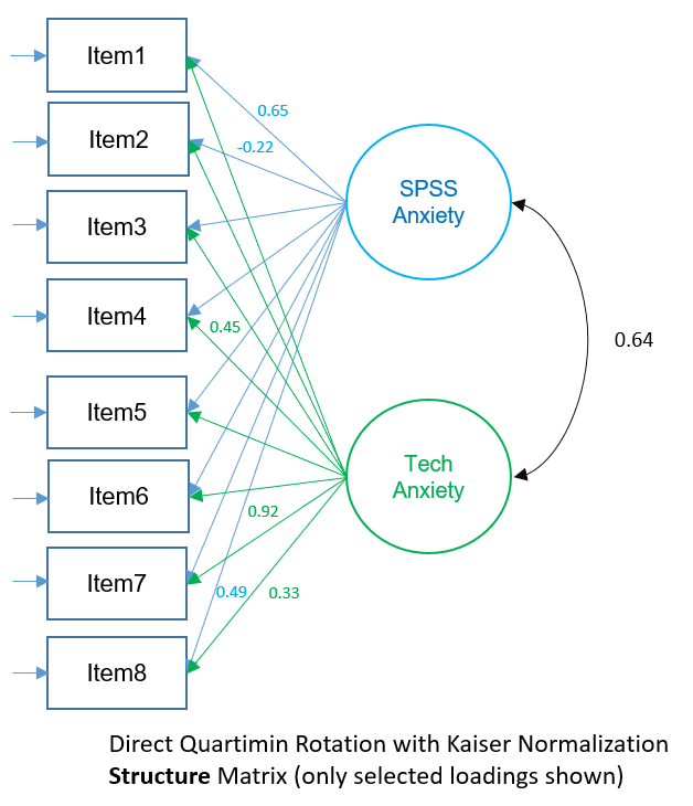
The factor structure matrix represent the simple zero-order correlations of the items with each factor (it’s as if you ran a simple regression where the single factor is the predictor and the item is the outcome). For example, \(0.653\) is the simple correlation of Factor 1 on Item 1 and \(0.333\) is the simple correlation of Factor 2 on Item 1. The more correlated the factors, the more difference between pattern and structure matrix and the more difficult to interpret the factor loadings. Looking at the Factor Pattern Matrix and using the absolute loading greater than 0.4 criteria, Items 1, 3, 4, 5 and 8 load highly onto Factor 1 and Items 6, and 7 load highly onto Factor 2 (bolded). Item 2 doesn’t seem to load well on either factor.
In the Factor Structure Matrix, we can look at the variance explained by each factor not controlling for the other factors. For example, Factor 1 contributes \((0.653)^2=0.426=42.6\%\) of the variance in Item 1, and Factor 2 contributes \((0.333)^2=0.11=11.0%\) of the variance in Item 1. Notice that the contribution in variance of Factor 2 is higher \(11\%\) vs. \(1.9\%\) because in the Pattern Matrix we controlled for the effect of Factor 1, whereas in the Structure Matrix we did not. In general, the loadings across the factors in the Structure Matrix will be higher than the Pattern Matrix because we are not partialling out the variance of the other factors.
| Factor | ||
| 1 | 2 | |
| Statistics makes me cry | .653 | .333 |
| My friends will think I’m stupid for not being able to cope with SPSS | -.222 | -.181 |
| Standard deviations excite me | -.559 | -.420 |
| I dream that Pearson is attacking me with correlation coefficients | .678 | .449 |
| I don’t understand statistics | .587 | .380 |
| I have little experience of computers | .398 | .553 |
| All computers hate me | .577 | .923 |
| I have never been good at mathematics | .485 | .330 |
| Extraction Method: Principal Axis Factoring. Rotation Method: Oblimin with Kaiser Normalization. | ||
The figure below shows the Structure Matrix depicted as a path diagram. Remember to interpret each loading as the zero-order correlation of the item on the factor (not controlling for the other factor).
Factor Correlation Matrix (2-factor PAF Direct Quartimin)
Recall that the more correlated the factors, the more difference between Pattern and Structure matrix and the more difficult it is to interpret the factor loadings. In our case, Factor 1 and Factor 2 are pretty highly correlated, which is why there is such a big difference between the factor pattern and factor structure matrices. Observe this in the Factor Correlation Matrix below.
| Factor | 1 | 2 |
| 1 | 1.000 | .636 |
| 2 | .636 | 1.000 |
| Extraction Method: Principal Axis Factoring. Rotation Method: Oblimin with Kaiser Normalization. | ||
Factor plot
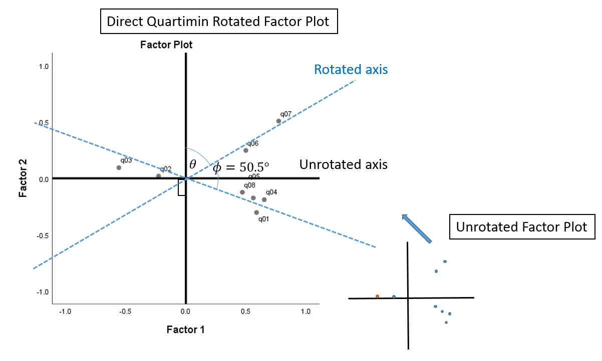
The difference between an orthogonal versus oblique rotation is that the factors in an oblique rotation are correlated. This means not only must we account for the angle of axis rotation \(\theta\), we have to account for the angle of correlation \(\phi\). The angle of axis rotation is defined as the angle between the rotated and unrotated axes (blue and black axes). From the Factor Correlation Matrix, we know that the correlation is \(0.636\), so the angle of correlation is \(cos^{-1}(0.636) = 50.5^{\circ}\), which is the angle between the two rotated axes (blue x and blue y-axis). The sum of rotations \(\theta\) and \(\phi\) is the total angle rotation. We are not given the angle of axis rotation, so we only know that the total angle rotation is \(\theta + \phi = \theta + 50.5^{\circ}\).
Compare the plot above with the Factor Plot in Rotated Factor Space from SPSS. You can see that if we “fan out” the blue rotated axes in the previous figure so that it appears to be \(90^{\circ}\) from each other, we will get the (black) x and y-axes for the Factor Plot in Rotated Factor Space. The difference between the figure below and the figure above is that the angle of rotation \(\theta\) is assumed and we are given the angle of correlation \(\phi\) that’s “fanned out” to look like it’s \(90^{\circ}\) when it’s actually not.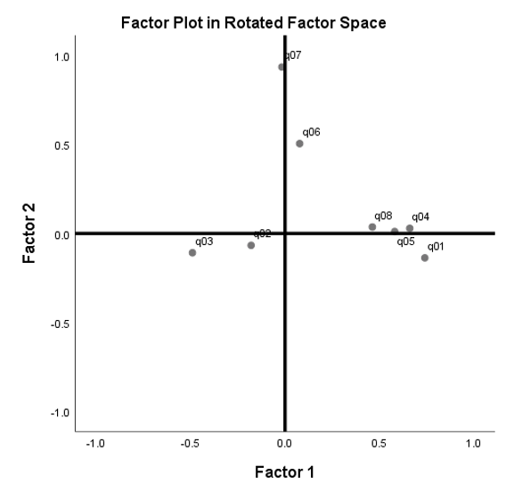
Relationship between the Pattern and Structure Matrix
The structure matrix is in fact derived from the pattern matrix. If you multiply the pattern matrix by the factor correlation matrix, you will get back the factor structure matrix. Let’s take the example of the ordered pair \((0.740,-0.137)\) from the Pattern Matrix, which represents the partial correlation of Item 1 with Factors 1 and 2 respectively. Performing matrix multiplication for the first column of the Factor Correlation Matrix we get
$$ (0.740)(1) + (-0.137)(0.636) = 0.740 – 0.087 =0.652.$$
Similarly, we multiple the ordered factor pair with the second column of the Factor Correlation Matrix to get:
$$ (0.740)(0.636) + (-0.137)(1) = 0.471 -0.137 =0.333 $$
Looking at the first row of the Structure Matrix we get \((0.653,0.333)\) which matches our calculation! This neat fact can be depicted with the following figure:
As a quick aside, suppose that the factors are orthogonal, which means that the factor correlations are 1′ s on the diagonal and zeros on the off-diagonal, a quick calculation with the ordered pair \((0.740,-0.137)\)
$$ (0.740)(1) + (-0.137)(0) = 0.740$$
and similarly,
$$ (0.740)(0) + (-0.137)(1) = -0.137$$
and you get back the same ordered pair. This is called multiplying by the identity matrix (think of it as multiplying \(2*1 = 2\)).
Questions
- Without changing your data or model, how would you make the factor pattern matrices and factor structure matrices more aligned with each other?
- True or False, When you decrease delta, the pattern and structure matrix will become closer to each other.
Answers: 1. Decrease the delta values so that the correlation between factors approaches zero. 2. T, the correlations will become more orthogonal and hence the pattern and structure matrix will be closer.
Total Variance Explained (2-factor PAF Direct Quartimin)
The column Extraction Sums of Squared Loadings is the same as the unrotated solution, but we have an additional column known as Rotation Sums of Squared Loadings. SPSS says itself that “when factors are correlated, sums of squared loadings cannot be added to obtain total variance”. You will note that compared to the Extraction Sums of Squared Loadings, the Rotation Sums of Squared Loadings is only slightly lower for Factor 1 but much higher for Factor 2. This is because unlike orthogonal rotation, this is no longer the unique contribution of Factor 1 and Factor 2. How do we obtain the Rotation Sums of Squared Loadings? SPSS squares the Structure Matrix and sums down the items.
| Factor | Extraction Sums of Squared Loadings | Rotation Sums of Squared Loadingsa | ||
| Total | % of Variance | Cumulative % | Total | |
| 1 | 2.511 | 31.382 | 31.382 | 2.318 |
| 2 | .499 | 6.238 | 37.621 | 1.931 |
| Extraction Method: Principal Axis Factoring. | ||||
| a. When factors are correlated, sums of squared loadings cannot be added to obtain a total variance. | ||||
As a demonstration, let’s obtain the loadings from the Structure Matrix for Factor 1
$$ (0.653)^2 + (-0.222)^2 + (-0.559)^2 + (0.678)^2 + (0.587)^2 + (0.398)^2 + (0.577)^2 + (0.485)^2 = 2.318.$$
Note that \(2.318\) matches the Rotation Sums of Squared Loadings for the first factor. This means that the Rotation Sums of Squared Loadings represent the non-unique contribution of each factor to total common variance, and summing these squared loadings for all factors can lead to estimates that are greater than total variance.
Interpreting the factor loadings (2-factor PAF Direct Quartimin)
Finally, let’s conclude by interpreting the factors loadings more carefully. Let’s compare the Pattern Matrix and Structure Matrix tables side-by-side. First we bold the absolute loadings that are higher than 0.4. We see that the absolute loadings in the Pattern Matrix are in general higher in Factor 1 compared to the Structure Matrix and lower for Factor 2. This makes sense because the Pattern Matrix partials out the effect of the other factor. Looking at the Pattern Matrix, Items 1, 3, 4, 5, and 8 load highly on Factor 1, and Items 6 and 7 load highly on Factor 2. Looking at the Structure Matrix, Items 1, 3, 4, 5, 7 and 8 are highly loaded onto Factor 1 and Items 3, 4, and 7 load highly onto Factor 2. Item 2 doesn’t seem to load on any factor. The results of the two matrices are somewhat inconsistent but can be explained by the fact that in the Structure Matrix Items 3, 4 and 7 seem to load onto both factors evenly but not in the Pattern Matrix. For this particular analysis, it seems to make more sense to interpret the Pattern Matrix because it’s clear that Factor 1 contributes uniquely to most items in the SAQ-8 and Factor 2 contributes common variance only to two items (Items 6 and 7). There is an argument here that perhaps Item 2 can be eliminated from our survey and to consolidate the factors into one SPSS Anxiety factor. We talk to the Principal Investigator and we think it’s feasible to accept SPSS Anxiety as the single factor explaining the common variance in all the items, but we choose to remove Item 2, so that the SAQ-8 is now the SAQ-7.
| Structure Matrix Pattern Matrix | ||||
| 1 | 2 | 1 | 2 | |
| Statistics makes me cry | .653 | .333 | .740 | -.137 |
| My friends will think I’m stupid for not being able to cope with SPSS | -.222 | -.181 | -.180 | -.067 |
| Standard deviations excite me | -.559 | -.420 | -.490 | -.108 |
| I dream that Pearson is attacking me with correlation coefficients | .678 | .449 | .660 | .029 |
| I don’t understand statistics | .587 | .380 | .580 | .011 |
| I have little experience of computers | .398 | .553 | .077 | .504 |
| All computers hate me | .577 | .923 | -.017 | .933 |
| I have never been good at mathematics | .485 | .330 | .462 | .036 |
| Extraction Method: Principal Axis Factoring. Rotation Method: Oblimin with Kaiser Normalization. | ||||
Quiz
True or False
- In oblique rotation, an element of a factor pattern matrix is the unique contribution of the factor to the item whereas an element in the factor structure matrix is the non-unique contribution to the factor to an item.
- In the Total Variance Explained table, the Rotation Sum of Squared Loadings represent the unique contribution of each factor to total common variance.
- The Pattern Matrix can be obtained by multiplying the Structure Matrix with the Factor Correlation Matrix
- If the factors are orthogonal, then the Pattern Matrix equals the Structure Matrix
- In oblique rotations, the sum of squared loadings for each item across all factors is equal to the communality (in the SPSS Communalities table) for that item.
Answers: 1. T, 2. F, represent the non-unique contribution (which means the total sum of squares can be greater than the total communality), 3. F, the Structure Matrix is obtained by multiplying the Pattern Matrix with the Factor Correlation Matrix, 4. T, it’s like multiplying a number by 1, you get the same number back, 5. F, this is true only for orthogonal rotations, the SPSS Communalities table in rotated factor solutions is based off of the unrotated solution, not the rotated solution.
Evaluating Simple Structure
As a special note, did we really achieve simple structure? Although rotation helps us achieve simple structure, if the interrelationships do not hold itself up to simple structure, we can only modify our model. In this case we chose to remove Item 2 from our model.
Promax Rotation
Promax is an oblique rotation method that begins with Varimax (orthgonal) rotation, and then uses Kappa to raise the power of the loadings. Promax really reduces the small loadings. Promax also runs faster than Direct Oblimin, and in our example Promax took 3 iterations while Direct Quartimin (Direct Oblimin with Delta =0) took 5 iterations.
Quiz
True or False
- Varimax, Quartimax and Equamax are three types of orthogonal rotation and Direct Oblimin, Direct Quartimin and Promax are three types of oblique rotations.
Answers: 1. T.
Generating Factor Scores
Suppose the Principal Investigator is happy with the final factor analysis which was the two-factor Direct Quartimin solution. She has a hypothesis that SPSS Anxiety and Attribution Bias predict student scores on an introductory statistics course, so would like to use the factor scores as a predictor in this new regression analysis. Since a factor is by nature unobserved, we need to first predict or generate plausible factor scores. In SPSS, there are three methods to factor score generation, Regression, Bartlett, and Anderson-Rubin.
Generating factor scores using the Regression Method in SPSS
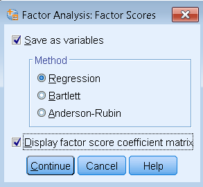
In order to generate factor scores, run the same factor analysis model but click on Factor Scores (Analyze – Dimension Reduction – Factor – Factor Scores). Then check Save as variables, pick the Method and optionally check Display factor score coefficient matrix.
The code pasted in the SPSS Syntax Editor looksl like this:
FACTOR
  /VARIABLES q01 q02 q03 q04 q05 q06 q07 q08
  /MISSING LISTWISE
  /ANALYSIS q01 q02 q03 q04 q05 q06 q07 q08
  /PRINT INITIAL EXTRACTION ROTATION FSCORE
  /PLOT EIGEN ROTATION
  /CRITERIA FACTORS(2) ITERATE(100)
  /EXTRACTION PAF
  /CRITERIA ITERATE(100) DELTA(0)
  /ROTATION OBLIMIN
  /SAVE REG(ALL)
  /METHOD=CORRELATION.
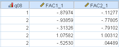
Here we picked the Regression approach after fitting our two-factor Direct Quartimin solution. After generating the factor scores, SPSS will add two extra variables to the end of your variable list, which you can view via Data View. The figure below shows what this looks like for the first 5 participants, which SPSS calls FAC1_1 and FAC2_1 for the first and second factors. These are now ready to be entered in another analysis as predictors.
For those who want to understand how the scores are generated, we can refer to the Factor Score Coefficient Matrix. These are essentially the regression weights that SPSS uses to generate the scores. We know that the ordered pair of scores for the first participant is \(-0.880, -0.113\). We also know that the 8 scores for the first participant are \(2, 1, 4, 2, 2, 2, 3, 1\). However, what SPSS uses is actually the standardized scores, which can be easily obtained in SPSS by using Analyze – Descriptive Statistics – Descriptives – Save standardized values as variables. The standardized scores obtained are: \(-0.452, -0.733, 1.32, -0.829, -0.749, -0.2025, 0.069, -1.42\).
Using the Factor Score Coefficient matrix, we multiply the participant scores by the coefficient matrix for each column. For the first factor:
$$ \begin{eqnarray} &(0.284) (-0.452) + (-0.048)(-0.733) + (-0.171)(1.32) + (0.274)(-0.829) \\ &+ (0.197)(-0.749) +(0.048)(-0.2025) + (0.174) (0.069) + (0.133)(-1.42) \\ &= -0.880, \end{eqnarray} $$
which matches FAC1_1 for the first participant. For the second factor FAC2_1 (the number is slightly different due to rounding error):
$$ \begin{eqnarray} &(0.005) (-0.452) + (-0.019)(-0.733) + (-0.045)(1.32) + (0.045)(-0.829) \\ &+ (0.036)(-0.749) +(0.095)(-0.2025) + (0.814) (0.069) + (0.028)(-1.42) \\ &= -0.115, \end{eqnarray} $$
| Factor | ||
| 1 | 2 | |
| Statistics makes me cry | .284 | .005 |
| My friends will think I’m stupid for not being able to cope with SPSS | -.048 | -.019 |
| Standard deviations excite me | -.171 | -.045 |
| I dream that Pearson is attacking me with correlation coefficients | .274 | .045 |
| I don’t understand statistics | .197 | .036 |
| I have little experience of computers | .048 | .095 |
| All computers hate me | .174 | .814 |
| I have never been good at mathematics | .133 | .028 |
| Extraction Method: Principal Axis Factoring. Rotation Method: Oblimin with Kaiser Normalization. Factor Scores Method: Regression. | ||
The second table is the Factor Score Covariance Matrix:
| Factor | 1 | 2 |
| 1 | 1.897 | 1.895 |
| 2 | 1.895 | 1.990 |
| Extraction Method: Principal Axis Factoring. Rotation Method: Oblimin with Kaiser Normalization. Factor Scores Method: Regression. | ||
This table can be interpreted as the covariance matrix of the factor scores, however it would only be equal to the raw covariance if the factors are orthogonal. For example, if we obtained the raw covariance matrix of the factor scores we would get
| REGR factor score 1 for analysis 1 | REGR factor score 2 for analysis 1 | ||
| REGR factor score 1 for analysis 1 | Covariance | .777 | .604 |
| REGR factor score 2 for analysis 1 | Covariance | .604 | .870 |
You will notice that these values are much lower. Let’s compare the same two tables but for Varimax rotation:
| Factor | 1 | 2 |
| 1 | .831 | .114 |
| 2 | .114 | .644 |
| Extraction Method: Principal Axis Factoring. Rotation Method: Varimax without Kaiser Normalization. Factor Scores Method: Regression. | ||
If you compare these elements to the Covariance table below, you will notice they are the same.
| REGR factor score 1 for analysis 2 | REGR factor score 2 for analysis 2 | ||
| REGR factor score 1 for analysis 2 | Covariance | .831 | .114 |
| REGR factor score 2 for analysis 2 | Covariance | .114 | .644 |
Note with the Bartlett and Anderson-Rubin methods you will not obtain the Factor Score Covariance matrix.
Regression, Bartlett and Anderson-Rubin compared
Among the three methods, each has its pluses and minuses. The Regression method produces scores that have a mean of zero and a variance equal to the squared multiple correlation between estimated and true factor scores. This maximizes the correlation between these two scores (and hence validity) but the scores can be somewhat biased. This means even if you use an orthogonal rotation like Varimax, you can still have correlated factor scores. For Bartlett’s method, the factor scores highly correlate with its own factor and not with others, and they are an unbiased estimate of the true factor score. Unbiased scores means that with repeated sampling of the factor scores, the average of the predicted scores is equal to the true factor score. The Anderson-Rubin method perfectly scales the factor scores so that the estimated factor scores are uncorrelated with other factors and uncorrelated with other estimated factor scores. Since Anderson-Rubin scores impose a correlation of zero between factor scores, it is not the best option to choose for oblique rotations. Additionally, Anderson-Rubin scores are biased.
In summary, if you do an orthogonal rotation, you can pick any of the the three methods. For orthogonal rotations, use Bartlett if you want unbiased scores, use the Regression method if you want to maximize validity and use Anderson-Rubin if you want the factor scores themselves to be uncorrelated with other factor scores. If you do oblique rotations, it’s preferable to stick with the Regression method. Do not use Anderson-Rubin for oblique rotations.
Quiz
True or False
- If you want the highest correlation of the factor score with the corresponding factor (i.e., highest validity), choose the regression method.
- Bartlett scores are unbiased whereas Regression and Anderson-Rubin scores are biased.
- Anderson-Rubin is appropriate for orthogonal but not for oblique rotation because factor scores will be uncorrelated with other factor scores.
Answers: 1. T, 2. T, 3. T

