This page has been updated!
Please refer to Confirmatory Factor Analysis (CFA) in R with lavaan for a much more thorough introduction to CFA.
II. Confirmatory Factor Analysis
- Introduction
- One factor CFA
- Identification
- Model fit
- Two factor CFA
- Uncorrelated Factors
- Correlated Factors
Back to Launch Page
Introduction
Confirmatory factor analysis borrows many of the same concepts from exploratory factor analysis except that instead of letting the data tell us the factor structure, we pre-determine the factor structure and perform a hypothesis test to see if this is true. In this portion of the seminar, we will continue with the example of the SAQ. However, from the exploratory factor analysis and talking to the Principal Investigator, we decided to remove Item 2 from the analysis. We will call this new survey the SAQ-7. Recall that this model assumes that SPSS Anxiety explains the common variance among all items (in this case seven) in the SAQ-7. In order to use the same file in Mplus you have to convert it to the CSV file version. Download here: saq8.csv
Let’s list the 7 items in the SAQ-7 (Item 2 was deleted and italicized):
- I dream that Pearson is attacking me with correlation coefficients
- I don’t understand statistics
- I have little experience of computers
- All computers hate me
- I have never been good at mathematics
- My friends are better at statistics than me
- Computers are useful only for playing games
- I did badly at mathematics at school
Recall from our exploratory analysis that Items 1,2,3,4,5, and 8 load onto each other and Items 6 and 7 load onto the same factor. As an exercise, let’s first assume that SPSS Anxiety is the only factor that explains common variance in all 7 items.
1. One Factor Confirmatory Factor Analysis
The most fundamental model in CFA is the one factor model, which will assume that the covariance (or correlation) among items is due to a single common factor. Much like exploratory common factor analysis, we will assume that total variance can be partitioned into common and unique variance.
In Mplus the code is relatively simple, note the BY statement indicates the items to the right of the statement loading onto the factor to the left of the statement.
TITLE: One Factor CFA SAQ-7 (Marker Method)
DATA: FILE IS saq8.csv;
VARIABLE: NAMES ARE q01-q08;
USEVARIABLES q01 q03-q08;
ANALYSIS: ESTIMATOR = ML;
MODEL: f1 BY q01 q03-q08;
OUTPUT: STDYX;
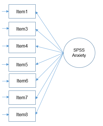
Graphically, this is what it looks like:

Model Fit Statistics
The three main model fit indices in CFA are:
- Model chi-square this is the chi-square statistic we obtain from the maximum likelihood statistic (similar to the EFA)
- CFI is the comparative fit index – values can range between 0 and 1 (values greater than 0.90, conservatively 0.95 indicate good fit)
- RMSEA is the root mean square error of approximation (values of 0.01, 0.05 and 0.08 indicate excellent, good and mediocre fit respectively, some go up to 0.10 for mediocre).
- In Mplus, you also obtain a p-value of close fit, that the RMSEA < 0.05. If you reject the model, it means your model is not a close fitting model.
Mplus lists another fit statistic along with the CFI called the TLI Tucker Lewis Index which also ranges between 0 and 1 with values greater than 0.90 indicating good fit. If the CFI and TLI are less than one, the CFI is always greater than the TLI.
In our one factor solution, we see that the chi-square is rejected. This usually happens for large samples (in this case we have N=2571). The RMSEA is 0.100 which indicates mediocre fit. The CFI is 0.906 and the TLI is 0.859, almost but not quite at the threshold of 0.95 and 0.90.
Chi-Square Test of Model Fit

          Value                            376.321
          Degrees of Freedom                    14
          P-Value                           0.0000

RMSEA (Root Mean Square Error Of Approximation)

          Estimate                           0.100
          90 Percent C.I.                    0.092  0.109
          Probability RMSEA <= .05           0.000

CFI/TLI

          CFI                                0.906
          TLI                                0.859
Identification of a CFA model (with at least three items)
In order to identify each factor in a CFA model with at least three indicators, there are two options:
- Set the variance of each factor to 1 (variance standardization method)
- Set the first loading of each factor to 1 (marker method)
Mplus by default uses Option 2, marker method if nothing else is specified.
TITLE: One Factor CFA Identifying Variance = 1
DATA: FILE IS saq8.csv;
VARIABLE: NAMES ARE q01-q08;
USEVARIABLES q01 q03-q08;
ANALYSIS: ESTIMATOR = ML;
MODEL: f1 BY q01* q03-q08;
f1 @1;
OUTPUT: STDYX;
                                                    Two-Tailed
                    Estimate       S.E.  Est./S.E.    P-Value
 F1       BY
    Q01                0.489      0.017     28.804      0.000
    Q03               -0.594      0.022    -26.953      0.000
    Q04                0.637      0.019     33.875      0.000
    Q05                0.556      0.020     28.218      0.000
    Q06                0.557      0.024     23.274      0.000
    Q07                0.714      0.022     31.809      0.000
    Q08                0.429      0.018     23.529      0.000

 Variances
    F1                 1.000      0.000    999.000    999.000
Below we show the STDYX solution, note that the loadings are different but the variances are the same.
STDYX Standardization
                                                    Two-Tailed
                    Estimate       S.E.  Est./S.E.    P-Value

 F1       BY
    Q01                0.590      0.016     36.337      0.000
    Q03               -0.553      0.017    -33.115      0.000
    Q04                0.672      0.014     46.439      0.000
    Q05                0.576      0.016     35.319      0.000
    Q06                0.497      0.018     27.130      0.000
    Q07                0.648      0.015     41.955      0.000
    Q08                0.491      0.018     27.557      0.000

Variances
    F1                 1.000      0.000    999.000    999.000
The STDYX solution standardizes the loading by the standard deviation of both the predictor (the factor, X) and the outcome (the item, Y). In the variance standardization method above, we only standardize by the predictor (the factor, X). In order to match the STDYX and variance standardization solutions, let’s first get the standard deviation of our outcome q01. Mplus only provides the variance, so we have the square root this to get the standard deviation.
	Variable/         Mean/
	Sample Size      Variance
Q01                       2.374
	   2571.000       0.685
The variance is \(0.685\); to get the standard deviation we square root to get \(\sqrt{0.685}=0.828\). In order to get the unstandardized solution to match STDYX, we take the loading and divide it by the standard deviation of q01, \(0.489/0.828=0.590\).
2. Two Factor Confirmatory Factor Analysis
Although the results from the one-factor CFA suggest that a one factor solution may capture much of the variance in these items, the model fit suggests that this model can be improved. From the exploratory factor analysis, we found that Items 6 and 7 “hang” together. Let’s take a look at Items 6 and 7 more carefully.
- Item 6: My friends are better at statistics than me
- Item 7: Computers are useful only for playing games
From talking to the Principal Investigator, it appears that these items constitute some sort of attribution bias, so we will name the factor as such.
Uncorrelated factors
We will now proceed with a two-factor CFA where we assume uncorrelated (or orthogonal) factors. Having a two-item factor presents a special problem for identification. In order to identify a two-item factor there are two options:
- Freely estimate the loadings of the two items on the same factor but equate them to be equal while setting the variance of the factor at 1
- Freely estimate the variance of the factor, using the marker method for the first item, but covary (correlate) the two-item factor with another factor
Since we are doing an uncorrelated two-factor solution here, we are relegated to the first option. One more snag is that Mplus by default correlates factors in a CFA, so you can turn off the correlation by specifying f1 with f2 @ 0. We continue to request the standardized loadings.
TITLE: Two Factor CFA SAQ-7 Factors Uncorrelated (Option 1)
DATA: FILE IS saq8.csv;
VARIABLE: NAMES ARE q01-q08;
USEVARIABLES q01 q03-q08;
ANALYSIS: ESTIMATOR = ML;
MODEL:
f1 BY q01* q03 q04 q05 q08;
f2 BY q06*(1)
 q07*(1);
f1 with f2 @ 0;
f1@1;
f2@1;
OUTPUT: STDYX;
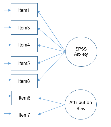
Here’s what the model looks like graphically:
Since we picked Option 1, we set the loadings to be equal to each other:
                                                    Two-Tailed
                    Estimate       S.E.  Est./S.E.    P-Value
F2       BY
    Q06                0.797      0.017     46.329      0.000
    Q07                0.797      0.017     46.329      0.000
We know the factors are uncorrelated because under MODEL RESULTS we see that F1 WITH F2 is estimated at zero, which is what we expect.
                                                    Two-Tailed
                    Estimate       S.E.  Est./S.E.    P-Value
 F1       WITH
    F2                 0.000      0.000    999.000    999.000
Looking at the MODEL FIT INFORMATION we see:
Chi-Square Test of Model Fit

          Value                            841.205
          Degrees of Freedom                    15
          P-Value                           0.0000

RMSEA (Root Mean Square Error Of Approximation)

          Estimate                           0.146
          90 Percent C.I.                    0.138  0.155
          Probability RMSEA <= .05           0.000

CFI/TLI

          CFI                                0.786
          TLI                                0.700
We can see that the uncorrelated two factor CFA solution gives us a higher chi-square (lower is better), higher RMSEA and lower CFI/TLI, which means overall it’s a poorer fitting model. We talk to the Principal Investigator and decide to go with a correlated (oblique) two factor model.
Correlated factors
We proceed with a correlated two-factor CFA. We still have the issue of that two-item factor; recall that for identification we can either equate the loadings and set the variance to 1 or we can covary the two-item factor with another factor and use the marker method. Taking advantage of our correlated factors, let’s use the second option. Looking at the code, it looks like everything is default in Mplus since Mplus automatically uses the marker method for both factors and automatically correlates the factors in a CFA.
TITLE: Two Factor CFA SAQ-7 Factors Correlated (Option 2)
DATA: FILE IS saq8.csv;
VARIABLE: NAMES ARE q01-q08;
USEVARIABLES q01 q03-q08;
ANALYSIS: ESTIMATOR = ML;
MODEL:
f1 BY q01 q03 q04 q05 q08;
f2 BY q06 q07;
OUTPUT: STDYX;
We use the marker method (setting the loading of the first item to 1) and freely estimate the variance. Notice that unlike Option 1, the first loading is not equal to the second loading.
                                                    Two-Tailed
                    Estimate       S.E.  Est./S.E.    P-Value
F2       BY
    Q06                1.000      0.000    999.000    999.000
    Q07                1.419      0.071     20.051      0.000
The marker method (Option 2) allows us to freely estimate the variances,
                                                    Two-Tailed
                    Estimate       S.E.  Est./S.E.    P-Value
Variances
    F1                 0.263      0.017     15.187      0.000
    F2                 0.447      0.033     13.496      0.000
but since we chose Option 2, we can covary (correlate) the two-item factor (Attribution Bias) with the five-item factor (SPSS anxiety), so we see that the covariance between the two factors is not zero.
                                                    Two-Tailed
                    Estimate       S.E.  Est./S.E.    P-Value
F2       WITH
    F1                 0.232      0.015     15.311      0.000
Let’s take a look at the MODEL FIT INFORMATION
Chi-Square Test of Model Fit

          Value                             66.768
          Degrees of Freedom                    13
          P-Value                           0.0000

RMSEA (Root Mean Square Error Of Approximation)

          Estimate                           0.040
          90 Percent C.I.                    0.031  0.050
          Probability RMSEA <= .05           0.952

CFI/TLI

          CFI                                0.986
          TLI                                0.977
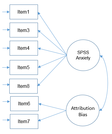
Notice that compared to the uncorrelated two-factor solution, the chi-square and RMSEA are both lower. The test of RMSEA is not significant which means that we do not reject the null hypothesis that the RMSEA is less than or equal to 0.05. Additionally the CFI and TLI are both higher and pass the 0.95 threshold. This is even better fitting than the one-factor solution. After talking with the Principal Investigator, we choose the final two correlated factor CFA model as shown below.


