- 1.1 Introduction to the SPSS Environment
- 1.2 A First Regression Analysis
- 1.3 Examining Data
- 1.4 Simple Linear Regression (Revisited)
- 1.5 Multiple Regression
- 1.6 Summary
- Go to Launch Page
1.1 Introduction to the SPSS Environment
Before we begin, let’s introduce three main windows that you will need to use to perform essential functions. The dataset used in this portion of the seminar is located here: elemapiv2
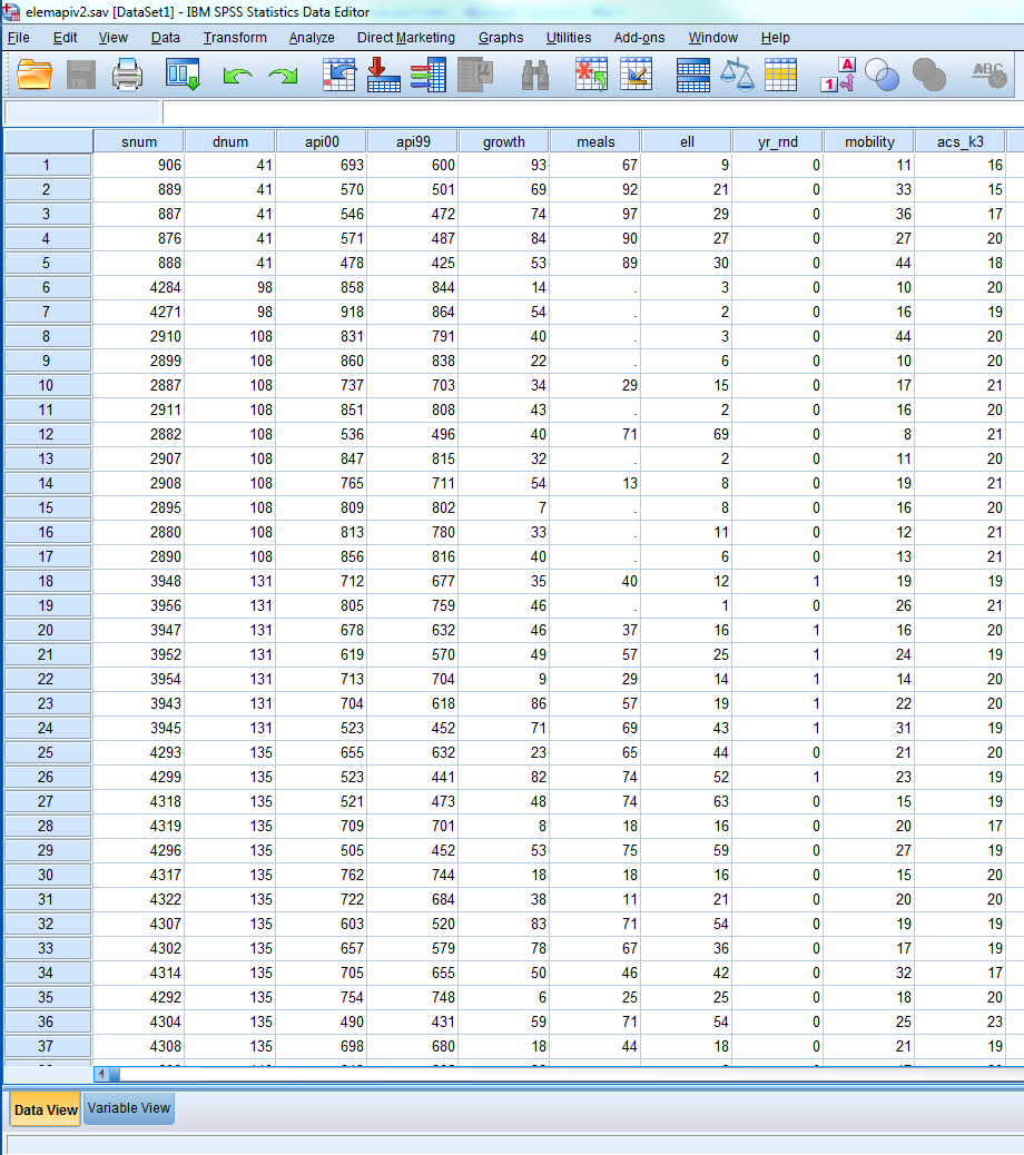
a) Data View
First is the Data View. This is like an Excel spreadsheet and should look familiar to you, except that the variable names are listed on the top row and the Case Numbers are listed row by row. You can enter or delete data directly as in Excel. If you delete data, these missing values in this dataset are represented by a dot.
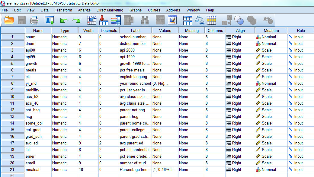
b) Variable View
The second is called Variable View, this is where you can view various components of your variables; but the important components are the Name, Label, Values and Measure. The Name specifies the name of your variable.
(Optional) The following attributes apply for SPSS variable names:
- They can be up to 64 characters long.
- SPSS is not case sensitive for variable names however it displays the case as you enter it.
- The first character must be a letter.
- Spaces between charcters are not allowed but the underscore _ is.
The Measure column is often overlooked but is important for certain analysis in SPSS and will help orient you to the type of analyses that are possible. You can choose between Scale, Ordinal or Nominal variables:
- Nominal: variables that have no intrinsic rating (e.g., gender, ethnicity)
- Ordinal: variables that have categories with an intrinsic ordering (e.g., Likert scales,Olympic medals)
- Scale: variables that are continuous with intrinsic ordering and meaningful metric (e.g., blood pressure, income)
In regression, you typically work with Scale outcomes and Scale predictors, although we will go into special cases of when you can use Nominal variables as predictors in Lesson 3.
From the Variable View we can see that we have 21 variables and the labels describing each of the variables. We will not go into all of the details about these variables. We have variables about academic performance in 2000 api00, and various characteristics of the schools, e.g., average class size in kindergarten to third grade acs_k3, parent’s education avg_ed, percent of teachers with full credentials full, and number of students enroll.
c) Syntax Editor
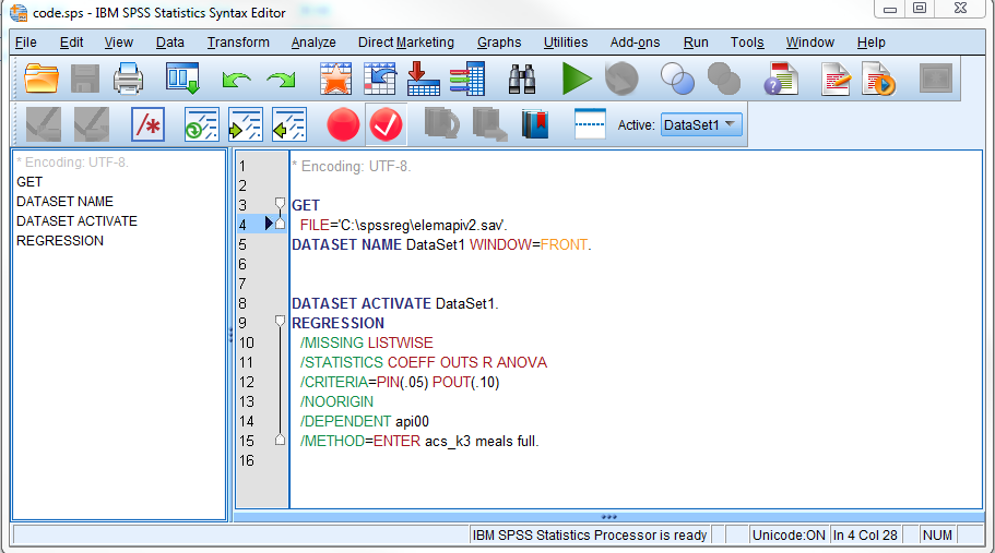
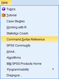
The Syntax Editor is where you enter SPSS Command Syntax. You can highlight portions of your code and implement it by pressing the Run Selection button. Note that you can explore all the syntax options in SPSS via the Command Syntax Reference by going to the Help menu. This will call a PDF file that is a reference for all the syntax available in SPSS.
As we will see in this seminar, there are some analyses you simply can’t do from the dialog box, which is why learning SPSS Command Syntax may be useful. Throughout this seminar, we will show you how to use both the dialog box and syntax when available. To begin, let’s go over basic syntax terminology:
- Command: instructions you give to SPSS to initiate an action (i.e., REGRESSION)
- Subcommand: addtional specficiations you give to the command, usually begins with a keyword and begin with a slash (i.e., /NOORIGIN), it can have specifications of its own (i.e., /METHOD=ENTER)
- Keyword: identifies the command, subcommands, and other specifications (i.e., TO, ALL)
- (Optional)
- Relational operator: a keyword that tells the relationship between two variables (EQ, GE, GT, LE, LT,NE)
- Logical operator: a keyword where you can create a truth table (AND, OR, NOT)
- Reserved keywords: a keyword particular to SPSS (ALL,BY,TO,WITH)
Note that a ** next to the specification means that it’s the default specification if no specification is provided (i.e., /MISSING = LISTWISE). When you paste the syntax from drop down menu, SPSS usually explicitly outputs the default specifications.
d) Viewer (Output) Window
After pasting the Syntax and clicking on the Run Selection button or by clicking OK from properly specifying your analysis through the menu system, you will see a new window pop up called the SPSS Viewer, otherwise known as the Output window. This is where all the results from your regression analysis will be stored.
Now that we are familiar with all the essential components of the SPSS environment, we can proceed to our first regression analysis.
1.2 A First Regression Analysis
The simple linear regression equation is
$$y_i = b_0 + b_1 x_i + e_i$$
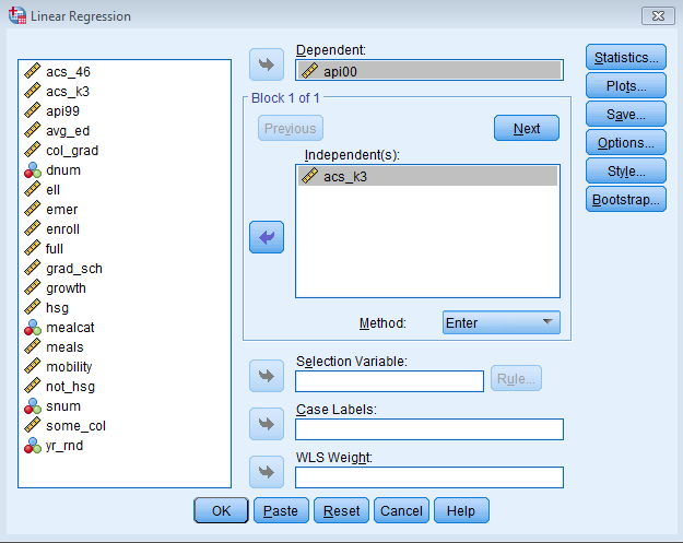
The index \(i\) can be a particular student, participant or observation. In this seminar, this index will be used for school. The term \(y_i\) is the dependent or outcome variable (e.g., api00) and \(x_i\) is the independent variable (e.g., acs_k3). The term \(b_0\) is the intercept, \(b_1\) is the regression coefficient, and \(e_i\) is the residual for each school. Now let’s run regression analysis using api00 as the dependent variable of academic performance. Let’s first include acs_k3 which is the average class size in kindergarten through 3rd grade (acs_k3). We expect that better academic performance would be associated with lower class size. Let’s try it first using the dialog box by going to Analyze – Regression – Linear
In the Linear Regression menu, you will see Dependent and Independent fields. Dependent variables are also known as outcome variables, which are variables that are predicted by the independent or predictor variables. Let’s not worry about the other fields for now. You can either click OK now, or click on Paste and you will see the code outputted in the Synatx Editor. Click the Run button to run the analysis.
This is the output that SPSS gives you if you paste the syntax.
	REGRESSION
	/MISSING LISTWISE
	/STATISTICS COEFF OUTS R ANOVA
	/CRITERIA=PIN(.05) POUT(.10)
	/NOORIGIN
	/DEPENDENT api00
	/METHOD=ENTER acs_k3.
| Model | Unstandardized Coefficients | Standardized Coefficients | t | Sig. | ||
| B | Std. Error | Beta | ||||
| 1 | (Constant) | 698.778 | 27.278 | 25.617 | .000 | |
| avg class size k-3 | -2.712 | 1.420 | -.096 | -1.910 | .057 | |
| a. Dependent Variable: api 2000 | ||||||
We omit certain portions of the output which we will discuss in detail later. Looking at the coefficients, the average class size (acs_k3, b=-2.712) is marginally significant (p = 0.057), and the coefficient is negative which would indicate that larger class sizes is related to lower academic performance — which is what we would expect. Should we take these results and write them up for publication? From these results, we would conclude that lower class sizes are related to higher performance. Before we write this up for publication, we should do a number of checks to make sure we can firmly stand behind these results. We start by getting more familiar with the data file, doing preliminary data checking, and looking for errors in the data.
1.3 Examining Data
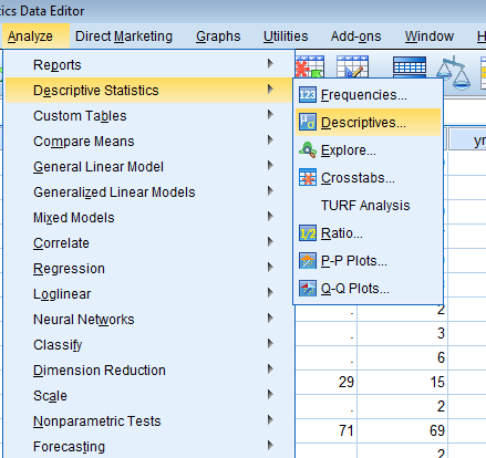
As researchers we need to make sure first that the data we cleaned hold plausible values. Let’s take a look at some descriptive information from our data set to determine whether the range of values is plausible. Go to Analyze – Descriptive Statistics – Descriptives.
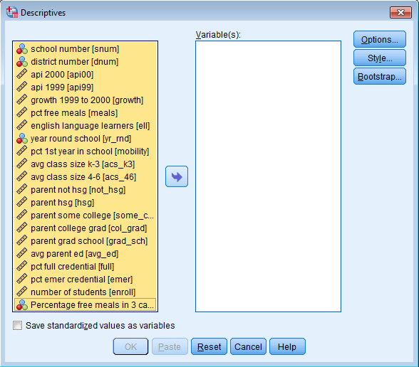
You will see two fields. Use your mouse and highlight the first variable, in this case snum, then while holding the Shift key (on a PC), click on the last variable you want your descriptives on, in this case mealcat. You should see the entire list of variables highlighted. Click on the right pointing arrow button and transfer the highlighted variables to the Variable(s) field. Click Paste.
You should get the following in the Syntax Editor.
	DESCRIPTIVES VARIABLES=snum dnum api00 api99
	growth meals ell yr_rnd mobility acs_k3 acs_46
	not_hsg hsg some_col col_grad grad_sch avg_ed full emer enroll mealcat
	/STATISTICS=MEAN STDDEV MIN MAX.
Equivalently, we can use the DESCRIPTIVES command with the keyword and specification /VAR=ALL to get descriptive statistics for all of the variables. The code is shown below:
DESCRIPTIVES /VAR=ALL.
| N | Minimum | Maximum | Mean | Std. Deviation | |
| school number | 400 | 58 | 6072 | 2866.81 | 1543.811 |
| district number | 400 | 41 | 796 | 457.73 | 184.823 |
| api 2000 | 400 | 369 | 940 | 647.62 | 142.249 |
| api 1999 | 400 | 333 | 917 | 610.21 | 147.136 |
| growth 1999 to 2000 | 400 | -69 | 134 | 37.41 | 25.247 |
| pct free meals | 315 | 6 | 100 | 71.99 | 24.386 |
| english language learners | 400 | 0 | 91 | 31.45 | 24.839 |
| year round school | 400 | 0 | 1 | .23 | .421 |
| pct 1st year in school | 399 | 2 | 47 | 18.25 | 7.485 |
| avg class size k-3 | 398 | -21 | 25 | 18.55 | 5.005 |
| avg class size 4-6 | 397 | 20 | 50 | 29.69 | 3.841 |
| parent not hsg | 400 | 0 | 100 | 21.25 | 20.676 |
| parent hsg | 400 | 0 | 100 | 26.02 | 16.333 |
| parent some college | 400 | 0 | 67 | 19.71 | 11.337 |
| parent college grad | 400 | 0 | 100 | 19.70 | 16.471 |
| parent grad school | 400 | 0 | 67 | 8.64 | 12.131 |
| avg parent ed | 381 | 1.00 | 4.62 | 2.6685 | .76379 |
| pct full credential | 400 | .42 | 100.00 | 66.0568 | 40.29793 |
| pct emer credential | 400 | 0 | 59 | 12.66 | 11.746 |
| number of students | 400 | 130 | 1570 | 483.47 | 226.448 |
| Percentage free meals in 3 categories | 400 | 1 | 3 | 2.02 | .819 |
| Valid N (listwise) | 295 |
Recall that we have 400 elementary schools in our subsample of the API 2000 data set. Some variables have missing values, like acs_k3 (average class size) which has a valid sample (N) of 398. When we did our original regression analysis the DF (degrees of freedom) Total was 397 (not shown above, see the ANOVA table in your output), which matches our expectation since the total degree of freedom in our Total Sums of Squares is the total sample size minus one. Taking a look at the minimum and maximum for acs_k3, the average class size ranges from -21 to 25. An average class size of -21 sounds implausible which means we need to investigate it further. Additionally, as we see from the Regression With SPSS web book, the variable full (pct full credential) appears to be entered in as proportions, hence we see 0.42 as the minimum. The last row in the Descriptives table, Valid N (listwise) is the sample size you would obtain if you put all the predictors of your table in your regression analysis, this is otherwise known as Listwise Deletion, which is the default implementation for the REGRESSION command. The descriptives have uncovered peculiarities worthy of further examination.
(Optional) Explore in SPSS
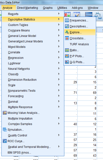
Let’s start with getting more detailed summary statistics for acs_k3 using the Explore function in SPSS. Go to Analyze – Descriptive Statistics – Explore.
You will see a dialog box appear as shown below. Note that you can right click on any white space region in the left hand side and click on Display Variable Names (additionally you can Sort Alphabetically, but this is not shown). Add the variable acs_k3 (average class size) into the Dependent List field by highlighting the variable on the left white field and clicking the right arrow button. Scale variables go into the Dependent List, and nominal variables go into the Factor List if you want to split the descriptives by particular levels of a nominal variable (e.g., school).
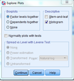
We want to see the univariate distribution of the average class size across schools. We can click on Analyze – Descriptive Statistics – Explore – Plots – Descriptive and uncheck Stem-and-leaf and check Histogram for us to output the histogram of acs_k3.
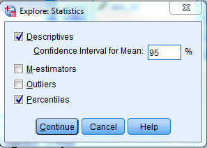
The actual values of the “fences” in the boxplots can be difficult to read. We can request percentiles to show where exactly the lines lie in the boxplot. Recall that the boxplot is marked by the 25th percentile on the bottom end and 75th percentile on the upper end. To request percentiles go to Analyze – Descriptive Statistics – Explore – Statistics.
The code you obtain from pasting the syntax
	EXAMINE VARIABLES=acs_k3
	/PLOT BOXPLOT HISTOGRAM
	/COMPARE GROUPS
	/PERCENTILES(5,10,25,50,75,90,95) HAVERAGE
	/STATISTICS DESCRIPTIVES
	/CINTERVAL 95
	/MISSING LISTWISE
	/NOTOTAL.
Now let’s take a look at the output.
| Cases | ||||||
| Valid | Missing | Total | ||||
| N | Percent | N | Percent | N | Percent | |
| avg class size k-3 | 398 | 99.5% | 2 | 0.5% | 400 | 100.0% |
We get Case Processing Summary which tells us again the Valid N and the number of missing, as expected.
| Statistic | Std. Error | |||
| avg class size k-3 | Mean | 18.55 | .251 | |
| 95% Confidence Interval for Mean | Lower Bound | 18.05 | ||
| Upper Bound | 19.04 | |||
| 5% Trimmed Mean | 19.13 | |||
| Median | 19.00 | |||
| Variance | 25.049 | |||
| Std. Deviation | 5.005 | |||
| Minimum | -21 | |||
| Maximum | 25 | |||
| Range | 46 | |||
| Interquartile Range | 2 | |||
| Skewness | -7.106 | .122 | ||
| Kurtosis | 53.014 | .244 | ||
The Descriptives output gives us detailed information about average class size. You can get special output that you can’t get from Analyze – Descriptive Statistics – Descriptives such as the 5% trimmed mean. Here are key points:
(Optional)
- The mean is 18.55 and the 95% Confidence Interval is (18.05,19.04). If we drew 100 samples of 400 schools from the population, we expect 95 of such intervals to contain the population mean.
- The 5% trimmed mean is the average class size we would obtain if we excluded the lower and upper 5% from our sample. If this value is very different from the mean we would expect outliers. In this case, since the trimmed mean is higher than the actual mean, the lowest observations seem to be pulling the actual mean down.
- The median (19.00) is the 50th percentile, which is the middle line of the boxplot. The Variance is how much variability we see in squared units, but for easier interpretation the Standard Deviation is the variability we see in average class size units. The closer the Standard Deviation is to zero the lower the variability.
- If the mean is greater than the median, it suggests a right skew, and conversely if the mean is less than the median it suggests a left skew. In this cass we have a left skew (which we will see in the histogram below).
- The minimum is -21 which again suggests implausible data. The maximum is 25 which is plausible.
- The range is the the difference between the maximum and minimum. The interquartile range is the difference between the 75th and 25th percentiles. It is also the upper and lower “fences” of the boxplot.
- Skewness is a measure of asymmetry, a threshold is 1 for positive skew and -1 for negative skew. The results indicate a high negative (left) skew.
- Kurtosis measures the heaviness of the the tails. Kurtosis values greater than 3 is considered not normal.
For more an annotated description of a similar analysis please see our web page: Annotated SPSS Output Descriptive statistics.
Histogram of Average Class Size
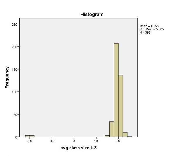
Let’s take a look now at the histogram which gives us a picture of the distribution of the average class size. Suppose we did not use SPSS Explore, then we can create a histogram through Graphs – Legacy Dialogs – Histogram. As we confirmed, the distribution is left skewed and we notice a particularly large outlier at -20. Note that histograms are in general better for depicting Scale variables.
Boxplot of Average Class Size
By default SPSS Explore will give you a boxplot. You can also go to Graphs – Legacy Dialogs – Boxplot – Simple and then choosing the “Summaries of separate variables” radio button, then clicking Define (note that the percentiles are not provided by default).
Boxplots are better for depicting Ordinal variables, since boxplots use percentiles as the indicator of central tendency and variability. The key percentiles to note are the 25, 50 and 75 since these indicate the lower, middle and upper “fences” on the boxplot. Note that Tukey’s hinges cannot take on fractional values whereas Weighted Average can.
| Percentiles | ||||||||
| 5 | 10 | 25 | 50 | 75 | 90 | 95 | ||
| Weighted Average(Definition 1) | avg class size k-3 | 16.00 | 17.00 | 18.00 | 19.00 | 20.00 | 21.00 | 21.00 |
| Tukey’s Hinges | avg class size k-3 | 18.00 | 19.00 | 20.00 | ||||
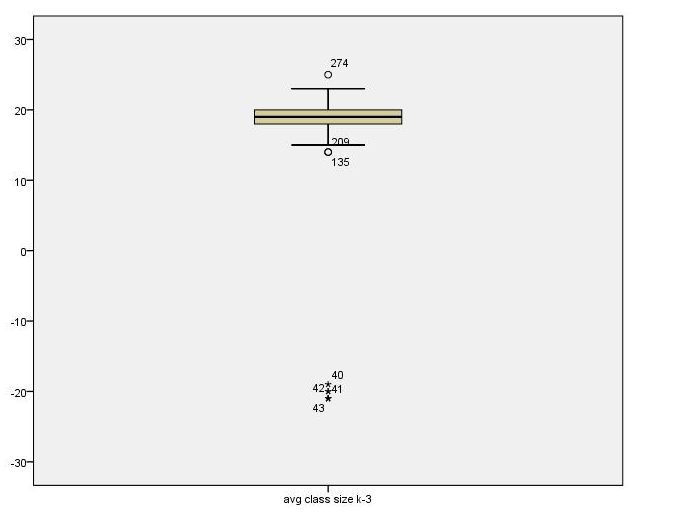
The boxplot is shown below. Pay particular attention to the circles which are mild outliers and stars, which indicate extreme outliers. Note that the extreme outliers are at the lower end.
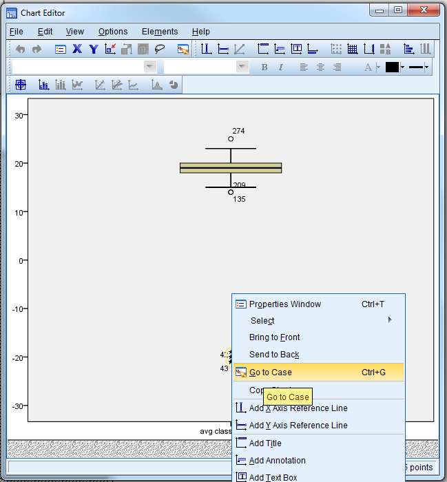
You can look at the outliers by double clicking on the boxplot and right click on the starred cases (extreme outliers). Then click on Go to Case to see the case in Data View.
Going back at Data View
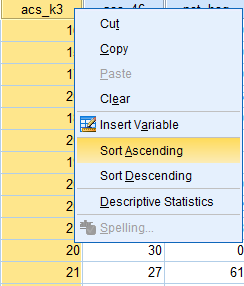
We see that the histogram and boxplot are effective in showing the schools with class sizes that are negative. Looking at the boxplot and histogram we see observations where the class sizes are around -21 and -20, so it seems as though some of the class sizes somehow became negative, as though a negative sign was incorrectly typed in front of them. To see if there’s a pattern, let’s look at the school and district number for these observations to see if they come from the same district. Indeed, they all come from district 140.
We can use Variable View to place variable acs_k3 from Position 10 to Position 3 by holding the left mouse button down on the left most column (in Windows) and dragging the variable up.
All of the observations from District 140 seem to have this problem. When you find such a problem, you want to go back to the original source of the data to verify the values. We have to reveal that we fabricated this error for illustration purposes, and that the actual data had no such problem. Let’s pretend that we checked with District 140 and there was a problem with the data there, a hyphen was accidentally put in front of the class sizes making them negative. We will make a note to fix this! Let’s continue checking our data.
Further steps
We recommend repeating these steps for all the variables you will be analyzing in your linear regression model. In particular, it seems there are additional typos in the full variable. In the Regression With SPSS web book we describe this error in more detail. In conclusion, we have identified problems with our original data which leads to incorrect conclusions about the effect of class size on academic performance. The corrected version of the data is called elemapi2v2. Let’s use that data file and repeat our analysis and see if the results are the same as our original analysis.
1.4 Simple Linear Regression (Revisited)
Now that we have the corrected data, we can proceed with the analysis! To simplify implementation, instead of using the SPSS menu system let’s try using Syntax Editor to run the code directly. If you leave out certain keywords specifications these are done by default SPSS such as /MISSING LISTWISE. Please go to Help – Command Syntax Reference for full details (note the **). Let’s use the REGRESSION command. The /DEPENDENT subcommand indicates the dependent variable, and the variables following /METHOD=ENTER are the predictors in the model (in this case we only have one predictor). Remember that predictors in Linear Regression are usually Scale variables such as age or height, but they may also be Nominal (e.g, ethnicity). The use of categorical variables will be covered in Lesson 3.
Now that we have the correct data, let’s revisit the relationship between average class size acs_k3 and academic performance api00.
	REGRESSION
	/MISSING LISTWISE
	/STATISTICS COEFF OUTS R ANOVA
	/CRITERIA=PIN(.05) POUT(.10)
	/NOORIGIN
	/DEPENDENT api00
	/METHOD=ENTER acs_k3.
| Model | R | R Square | Adjusted R Square | Std. Error of the Estimate |
| 1 | .171a | .029 | .027 | 140.165 |
| a. Predictors: (Constant), avg class size k-3 | ||||
| Model | Sum of Squares | df | Mean Square | F | Sig. | ||
| 1 | Regression | 234353.831 | 1 | 234353.831 | 11.929 | .001b | |
| Residual | 7779853.307 | 396 | 19646.094 | ||||
| Total | 8014207.138 | 397 | |||||
| a. Dependent Variable: api 2000 | |||||||
| b. Predictors: (Constant), avg class size k-3 | |||||||
| Model | Unstandardized Coefficients | Standardized Coefficients | t | Sig. | |||
| B | Std. Error | Beta | |||||
| 1 | (Constant) | 308.337 | 98.731 | 3.123 | .002 | ||
| avg class size k-3 | 17.751 | 5.140 | .171 | 3.454 | .001 | ||
| a. Dependent Variable: api 2000 | |||||||
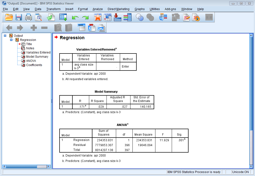
Looking at the Model Summary we see that the R square is .029, which means that approximately 2.9% of the variance of api00 is accounted for by the model. The R is the correlation of the model with the outcome, and since we only have one predictor, this is in fact the correlation of acs_k3 with api00. From the ANOVA table we see that the F-test and hence our model is statistically significant. Looking at the Coefficients table the constant or intercept term is 308.34, and this is the predicted value of academic performance when acs_k3 equals zero. We are not that interested in this coefficient because a class size of zero is not plausible. The t-test for acs_k3 equals 3.454, and is statistically significant, meaning that the regression coefficient for acs_k3 is significantly different from zero. Note that (3.454)2 = 11.93, which is the same as the F-statistic (with some rounding error). The coefficient for acs_k3 is 17.75, meaning that for a one student increase in average class size, we would expect a 17.75 increase in api00. Additionally from the Standardized Coefficients Beta, a one standard deviation increase in average class size leads to a 0.171 standard deviation increase in academic performance.
(Optional)Simple linear regression as correlation
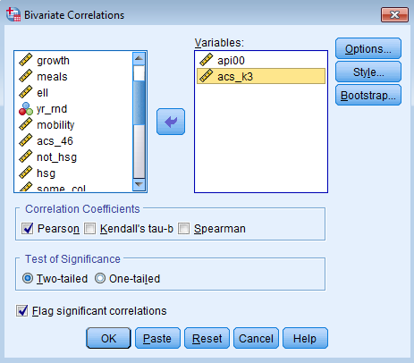
To understand the relationship between correlation and simple regression, let’s run a bivariate correlation of api00 and acs_k3 (average class size). Go to Analyze – Correlate – Bivariate.
Move api00 and acs_k3 from the left field to the right field by highlighting the two variables (holding down Ctrl on a PC) and then clicking on the right arrow.
The resulting syntax you obtain is as follows:
	CORRELATIONS
	/VARIABLES=api00 acs_k3
	/PRINT=TWOTAIL NOSIG
	/MISSING=PAIRWISE.
The resulting output you obtain is shown:
| api 2000 | avg class size k-3 | |||
| api 2000 | Pearson Correlation | 1 | .171** | |
| Sig. (2-tailed) | .001 | |||
| N | 400 | 398 | ||
| avg class size k-3 | Pearson Correlation | .171** | 1 | |
| Sig. (2-tailed) | .001 | |||
| N | 398 | 398 | ||
| **. Correlation is significant at the 0.01 level (2-tailed). | ||||
Note that the correlation is equal to the Standardized Coefficients Beta column from our simple linear regression, whose term we will denote \(\hat{\beta}\) with a hat to indicate that it’s being estimated from our sample.
The formula for an unstandardized coefficient in simple linear regression is:
$$\hat{b}_1=corr(y,x)* \frac{SD(y)}{SD(x)}.$$
For a standardized variable:
$$\hat{\beta_1}=corr(Z_y,Z_x)* \frac{SD(Z_y)}{SD(Z_x)}.$$
Since the standard deviation is for a standardized variable is 1, the terms on the right hand divide to 1 and we simply get the correlation coefficient. It can be shown that the correlation of the z-scores are the same as the correlation of the original variables:
$$\hat{\beta_1}=corr(Z_y,Z_x)=corr(y,x).$$
Thus, for simple linear regression, the standardized beta coefficients are simply the correlation of the two unstandardized variables!
1.5 Multiple Regression
The proportion of variance explained by average class size was only 2.9%. In order to improve the proportion variance accounted for by the model, we can add more predictors. A regression model that has more than one predictor is called multiple regression (don’t confuse it with multivariate regression which means you have more than one dependent variable). Let’s suppose we have three predictors, then the equation looks like:
$$y_i = b_0 + b_1 x_{1i} + b_2 x_{2i} + b_3 x_{3i} + e_i$$
For this multiple regression example, we will regress the dependent variable, api00, on predictors acs_k3, meals and full. We can modify the code directly from Section 1.4. Remember to use the corrected data file: elemapi2v2.
	REGRESSION
	/MISSING LISTWISE
	/STATISTICS COEFF OUTS R ANOVA
	/CRITERIA=PIN(.05) POUT(.10)
	/NOORIGIN
	/DEPENDENT api00
	/METHOD=ENTER acs_k3 meals full.
The output you obtain is as follows:
| Model | Variables Entered | Variables Removed | Method |
| 1 | pct full credential, avg class size k-3, pct free mealsb | . | Enter |
| a. Dependent Variable: api 2000 | |||
| b. All requested variables entered. | |||
| Model | R | R Square | Adjusted R Square | Std. Error of the Estimate |
| 1 | .908a | .824 | .823 | 59.806 |
| a. Predictors: (Constant), pct full credential, avg class size k-3, pct free meals | ||||
| Model | Sum of Squares | df | Mean Square | F | Sig. | ||
| 1 | Regression | 6604966.181 | 3 | 2201655.394 | 615.546 | .000b | |
| Residual | 1409240.958 | 394 | 3576.754 | ||||
| Total | 8014207.138 | 397 | |||||
| a. Dependent Variable: api 2000 | |||||||
| b. Predictors: (Constant), pct full credential, avg class size k-3, pct free meals | |||||||
| Model | Unstandardized Coefficients | Standardized Coefficients | t | Sig. | |||
| B | Std. Error | Beta | |||||
| 1 | (Constant) | 771.658 | 48.861 | 15.793 | .000 | ||
| avg class size k-3 | -.717 | 2.239 | -.007 | -.320 | .749 | ||
| pct free meals | -3.686 | .112 | -.828 | -32.978 | .000 | ||
| pct full credential | 1.327 | .239 | .139 | 5.556 | .000 | ||
| a. Dependent Variable: api 2000 | |||||||
Let’s examine the output from this regression analysis. As with the simple regression, we look to the p-value of the F-test to see if the overall model is significant. With a p-value of zero to three decimal places, the model is statistically significant. The R-squared is 0.824, meaning that approximately 82% of the variability of api00 is accounted for by the variables in the model. In this case, the adjusted R-squared indicates that about 82% of the variability of api00 is accounted for by the model, even after taking into account the number of predictor variables in the model. The coefficients for each of the variables indicates the amount of change one could expect in api00 given a one-unit change in the value of that variable, given that all other variables in the model are held constant. For example, consider the variable meals. We would expect a decrease of 3.686 in the api00 score for every one unit increase in percent free meals, assuming that all other variables in the model are held constant. The interpretation of much of the output from the multiple regression is the same as it was for the simple regression.
We see quite a difference in the coefficients compared to the simple linear regression. In the simple regression, acs_k3 was significantly positive B = 17.75, p < 0.01, with an R-square of .027. This suggests that increasing average class size increases academic performance (which is counterintuitive). When we add in full (percent of full credential teachers at the school) and meals (percent of free meals at school) we notice that the coefficient for avg_k3 is now B = -.717, p = 0.749 which means that the effect of class size on academic performance is not significant. We can do a check of collinearity to see if avg_k3 is collinear with the other predictors in our model (see Lesson 2: SPSS Regression Diagnostics). In this case however, it looks like meals, which is an indicator of socioeconomic status, is acting as a suppression variable (which we won’t cover in this seminar).
(Optional) You may be wondering what a -3.686 change in meals really means, and how you might compare the strength of that coefficient to the coefficient for another variable, say full. To address this problem, we can refer to the column Standardized Coefficients Beta, also known as standardized regression coefficients. The Beta coefficients are used by some researchers to compare the relative strength of the various predictors within the model. Because the Beta coefficients are all measured in standard deviations, instead of the units of the variables, they can be compared to one another. In other words, the beta coefficients are the coefficients that you would obtain if the outcome and predictor variables were all transformed to standard scores, also called z-scores, before running the regression. In this example, meals has the largest Beta coefficient, -0.828, and acs_k3 has the smallest Beta, -0.007. Thus, a one standard deviation increase in meals leads to a 0.828 standard deviation decrease in predicted api00, with the other variables held constant. And, a one standard deviation increase in acs_k3, in turn, leads to a -0.007 standard deviation decrease api00 with the other variables in the model held constant. This means that the positive relationship between average class size and academic performance can be explained away by adding a proxy of socioeconomic status and teacher quality into our model.
Adding student enrollment into our multiple regression model
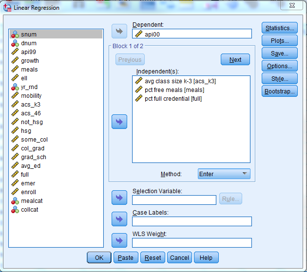
Suppose we want to see if adding student enrollment (enroll) adds any additional benefit to our model. Perhaps we should control for the size of the school itself in our analysis. We can perform what’s called a hierarchical regression analysis, which is just a series of linear regressions separated into what SPSS calls Blocks. In Block 1 let’s enter in the same predictors from our previous analysis.
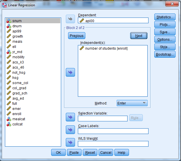
To see the additional benefit of adding student enrollment as a predictor let’s click Next and move on to Block 2. Remember that the previous predictors in Block 1 are also included in Block 2.
Note that we need to output something called the R squared change, so under Linear Regression click on Statistics and check the R squared change box and click Continue. The syntax looks like this (notice the new keyword CHANGE under the /STATISTICS subcommand).
REGRESSION
  /MISSING LISTWISE
  /STATISTICS COEFF OUTS R ANOVA CHANGE
  /CRITERIA=PIN(.05) POUT(.10)
  /NOORIGIN
  /DEPENDENT api00
  /METHOD=ENTER acs_k3 full meals
  /METHOD=ENTER enroll.
The output we obtain from this analysis is:
| Model | Variables Entered | Variables Removed | Method |
| 1 | pct full credential, avg class size k-3, pct free mealsb | . | Enter |
| 2 | number of studentsb | . | Enter |
| a. Dependent Variable: api 2000 | |||
| b. All requested variables entered. | |||
| Model | R | R Square | Adjusted R Square | Std. Error of the Estimate | Change Statistics | ||||
| R Square Change | F Change | df1 | df2 | Sig. F Change | |||||
| 1 | .908a | .824 | .823 | 59.806 | .824 | 615.546 | 3 | 394 | .000 |
| 2 | .911b | .830 | .828 | 58.860 | .006 | 13.772 | 1 | 393 | .000 |
| a. Predictors: (Constant), pct full credential, avg class size k-3, pct free meals | |||||||||
| b. Predictors: (Constant), pct full credential, avg class size k-3, pct free meals, number of students | |||||||||
| Model | Sum of Squares | df | Mean Square | F | Sig. | ||
| 1 | Regression | 6604966.181 | 3 | 2201655.394 | 615.546 | .000b | |
| Residual | 1409240.958 | 394 | 3576.754 | ||||
| Total | 8014207.138 | 397 | |||||
| 2 | Regression | 6652679.396 | 4 | 1663169.849 | 480.068 | .000c | |
| Residual | 1361527.742 | 393 | 3464.447 | ||||
| Total | 8014207.138 | 397 | |||||
| a. Dependent Variable: api 2000 | |||||||
| b. Predictors: (Constant), pct full credential, avg class size k-3, pct free meals | |||||||
| c. Predictors: (Constant), pct full credential, avg class size k-3, pct free meals, number of students | |||||||
| Model | Unstandardized Coefficients | Standardized Coefficients | t | Sig. | |||
| B | Std. Error | Beta | |||||
| 1 | (Constant) | 771.658 | 48.861 | 15.793 | .000 | ||
| avg class size k-3 | -.717 | 2.239 | -.007 | -.320 | .749 | ||
| pct free meals | -3.686 | .112 | -.828 | -32.978 | .000 | ||
| pct full credential | 1.327 | .239 | .139 | 5.556 | .000 | ||
| 2 | (Constant) | 785.555 | 48.233 | 16.287 | .000 | ||
| avg class size k-3 | .841 | 2.243 | .008 | .375 | .708 | ||
| pct free meals | -3.645 | .111 | -.819 | -32.965 | .000 | ||
| pct full credential | 1.080 | .244 | .113 | 4.420 | .000 | ||
| number of students | -.052 | .014 | -.084 | -3.711 | .000 | ||
| a. Dependent Variable: api 2000 | |||||||
| Model | Beta In | t | Sig. | Partial Correlation | Collinearity Statistics | ||
| Tolerance | |||||||
| 1 | number of students | -.084b | -3.711 | .000 | -.184 | .849 | |
| a. Dependent Variable: api 2000 | |||||||
| b. Predictors in the Model: (Constant), pct full credential, avg class size k-3, pct free meals | |||||||
We can see that adding student enrollment as a predictor results in an R square change of 0.006. This means that there is an increase of 0.6% in the proportion of variance explained by adding enroll. The change in F(1,393) = 13.772 is significant. Here’s where we would as a researcher determine whether a significant predictor results in practical significance. Notice that the sign of the average class size coefficient changes, although in both models it is not significant.
(Optional) Looking at the Standardized Coefficients Beta column an increase in one standard deviation enrolled results in a -.084 standard deviation decrease in academic performance. Additionally, we can consider dividing enroll by 100 to determine the effect of increasing student enrollment by 100 students on academic performance.
1.6 Summary
In this seminar we have discussed the basics of how to perform simple and multiple regressions, the basics of interpreting output, as well as some related commands. We examined some tools and techniques for screening for bad data and the consequences such data can have on your results. We began with a simple hypothesis that decreasing class size increases academic performance. However, what we realize is that a correct conclusion must first be based on valid data as well as a sufficiently specified model. Our initial findings were changed when we removed implausible (negative) values of average class size. After correcting the data, we arrived at the finding that just adding class size as the sole predictor results in a positive effect of increasing class size on academic performance. However the R-square was low. When we put in more explanatory predictors into our model such as proxies of socioeconomic status, teacher quality and school enrollment, the effect of class size disappeared. Our hypothesis that larger class size decreases performance was not confirmed when we specified the full model. Let’s move onto the next lesson where we make sure the assumptions of linear regression are satisfied in making our inferences.
(Optional) Proof for the Standardized Regression Coefficient for Simple Linear Regression
Suppose \(a\) and \(b\) are the unstandardized intercept and regression coefficient respectively in a simple linear regression model. Additionally, we are given that the formula for the intercept is \(a=\bar{y}-b_1 \bar{x}\). The simple linear equation is given as:
$$y_i=a+b_1x_i+\epsilon_i$$
Substituting the formula for the intercept we obtain:
$$y_i=(\bar{y}-b_1 \bar{x})+b_1x_i+\epsilon_i$$
Rearranging terms:
$$y_i=\bar{y}+b_1(x_i-\bar{x})+\epsilon_i$$
Subtract both sides by \(\bar{y}\), note the first term in the right hand side goes to zero:
$$(y_i-\bar{y})=(\bar{y}-\bar{y})+b_1(x_i-\bar{x})+\epsilon_i$$
Multiply the resulting first term in the right hand side by \(\frac{SD(x)}{SD(x)}=1\):
$$(y_i-\bar{y})=b_1\frac{(x_i-\bar{x})}{SD(x)}*{SD(x)}+\epsilon_i$$
Substitute \(Z_{x(i)} =(x_i-\bar{x})/SD(x)\), which is the standardized variable of \(x\):
$$(y_i-\bar{y})= b_1Z_{x(i)}*SD(x)+\epsilon_i$$
Divide both sides by \(SD(y)\):
$$\frac{(y_i-\bar{y})}{SD(y)}=(b_1*\frac{SD(x)}{SD(y)})Z_{x(i)}+\frac{\epsilon_i}{SD(y)}$$
Substitute \(Z_{y(i)} = (y_i-\bar{y})/SD(y)\), which is the standardized variable of \(y\), and \(\epsilon_i’=\epsilon_i/SD(y)\):
$$Z_{y(i)}=(b_1*\frac{SD(x)}{SD(y)})Z_{x(i)} +\epsilon_i’$$
Essentially, the equation above becomes a new simple regression equation where the intercept is zero (since the variables are centered) with a new regression coefficient (slope):
$$\beta_1 = b_1*\frac{SD(x)}{SD(y)}$$

