
- 2.0 Regression Diagnostics
- 2.1 Tests on Nonlinearity and Nonconstant Error of Variance
- 2.2 Tests on Normality of Residuals
- 2.3 Model Specification
- 2.4 Issues of Independence
- 2.5 Tests on Multicollinearity
- 2.6 Unusual and Influential data
- 2.7 Summary
- Go to Launch Page
2.0 Regression Diagnostics
In our last lesson, we learned how to first examine the distribution of variables before doing simple and multiple linear regressions with SPSS. Without verifying that your data has been entered correctly and checking for plausible values, your coefficients may be misleading. In a similar vein, failing to check for assumptions of linear regression can bias your estimated coefficients and
standard errors (e.g., you can get a significant effect when in fact there is none, or vice versa). This lesson will discuss how to check whether your data meet the assumptions of linear regression. Recall that the regression equation (for simple linear regression) is:
$$ y_i = b_0 + b_1 x_i + \epsilon_i$$
Additionally, we make the assumption that
$$ \epsilon_i \sim N(0, \sigma^2)$$
which says that the residuals are normally distributed with a mean centered around zero. Let’s take a look a what a residual and predicted value are visually:

The observations are represented by the circular dots, and the best fit or predicted regression line is represented by the diagonal solid line. The residual is the vertical distance (or deviation) from the observation to the predicted regression line. Predicted values are points that fall on the predicted line for a given point on the x-axis. In this particular case we plotting api00 with enroll. Since we have 400 schools, we will have 400 residuals or deviations from the predicted line.
Assumptions in linear regression are based mostly on predicted values and residuals. In particular, we will consider the following assumptions.
- Linearity – the relationships between the predictors and the outcome variable should be linear. Big deal if violated.
- Homogeneity of variance (homoscedasticity) – the error variance should be constant. Not as big deal if violated.
- Normality – the errors should be normally distributed – normality is necessary for the b-coefficient tests to be valid (especially for small samples), estimation of the coefficients only requires that the errors be identically and independently distributed. Not as big of a deal if violated.
- Independence – the errors associated with one observation are not correlated with the errors of any other observation. Huge deal if violated!
- Model specification – the model should be properly specified (including all relevant variables, and excluding irrelevant variables)
Additionally, there are issues that can arise during the analysis that, while strictly speaking are not assumptions of regression, are nonetheless, of great
concern to regression analysts.
- Multicollinearity – predictors that are highly related to each other and both predictive of your outcome, can cause problems in estimating the regression coefficients.
- Unusual and Influential Data
- Outliers: observations with large residuals (the deviation of the predicted score from the actual score), note that both the red and blue lines represent the distance of the outlier from the predicted line at a particular value of enroll
- Leverage: measures the extent to which the predictor differs from the mean of the predictor; the red residual has lower leverage than the blue residual
- Influence: observations that have high leverage and are extreme outliers, changes coefficient estimates drastically if not included
Many graphical methods and numerical tests have been developed over the years for regression diagnostics and SPSS makes many of these methods easy to access and use. In this lesson, we will explore these methods and show how to verify regression assumptions and detect potential problems using SPSS. We will use the same dataset elemapi2v2 (remember it’s the modified one!) that we used in Lesson 1. Our goal is to make the best predictive model of academic performance possible using a combination of predictors such as meals, acs_k3, full, and enroll.
Here is a table of the type of residuals we will be using for this seminar:
| Keyword | Description |
Assumption Checked |
| PRED | Unstandardized predicted values. |
Linearity, Homogeneity of Error Variance |
| ZPRED | Standardized predicted values. |
|
| RESID | Unstandardized residuals. | Linearity, Homogeneity of Error Variance, Outliers |
| ZRESID | Standardized residuals. |
|
| LEVER | Centered leverage values. |
Unusual and Influential Data |
| COOK | Cook’s distances. | |
| DFBETA | DF Beta |
Standardized variables (either the predicted values or the residuals) have a mean of zero and standard deviation of one. If residuals are normally distributed, then 95% of them should fall between -2 and 2. If they fall above 2 or below -2, they can be considered unusual.
2.1 Tests on Nonlinearity and Homogeneity of Variance
Testing Nonlinearity
When we do linear regression, we assume that the relationship between the response variable and the predictors is linear. If this assumption is violated, the linear regression will try to fit a straight line to data that do not follow a straight line. The bivariate plot of the predicted value against residuals can help us infer whether the relationships of the predictors to the outcome is linear. Let’s get the scatterplot of the standardized predicted value of api00 on enroll against the standardized residuals. First go to Analyze – Regression – Linear and shift api00 into the Dependent field and enroll in the Independent(s) field and click Continue. Then click on Plots. Shift *ZRESID to the Y: field and *ZPRED to the X: field, these are the standardized residuals and standardized predicted values respectively.
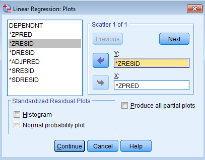
The code you obtain is:
	REGRESSION
	/MISSING LISTWISE
	/STATISTICS COEFF OUTS R ANOVA
	/CRITERIA=PIN(.05) POUT(.10)
	/NOORIGIN
	/DEPENDENT api00
	/METHOD=ENTER enroll
	/SCATTERPLOT=(*ZRESID ,*ZPRED).
We will ignore the regression tables for now since our primary concern is the scatterplot of the standardized residuals with the standardized predicted values. Let’s take a look at the scatterplot.
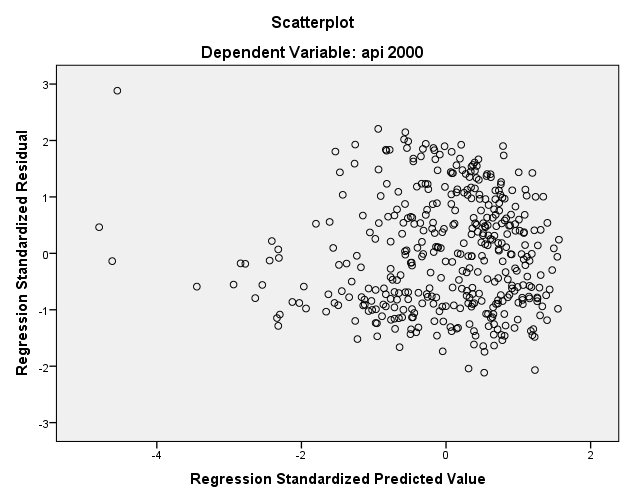
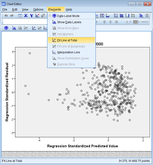
It’s difficult to tell the relationship simply from this plot. Let’s try fitting a non-linear best fit line known as the Loess Curve through the scatterplot to see if we can detect any nonlinearity. To do that double click on the scatterplot itself in the Output window go to Elements – Fit Line at Total.
You will see a menu system called Properties. Click Fit Line – Loess and Apply.
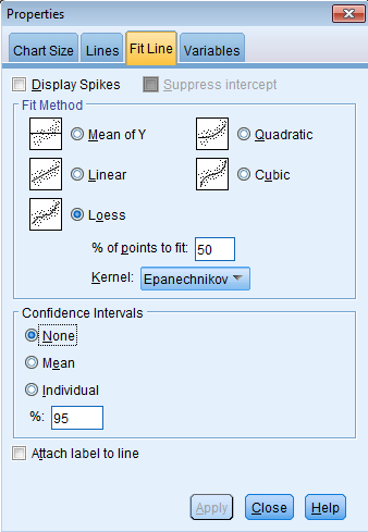
Your scatterplot of the standardized predicted value with the standardized residual will now have a Loess curve fitted through it. Note that this does not change our regression analysis, this only updates our scatterplot.

From the Loess curve, it appears that the relationship of standardized predicted to residuals is roughly linear around zero. We can conclude that the relationship between the response variable and predictors is zero since the residuals seem to be randomly scattered around zero.
Testing homogeneity of error variance
Another assumption of ordinary least squares regression is that the variance of the residuals is homogeneous across levels of the predicted values, also known as homoscedasticity. If the model is well-fitted, there should be no pattern to the residuals plotted against the fitted values. If the variance of the residuals is non-constant then the residual variance is said to be heteroscedastic. Just as for the assessment of linearity, a commonly used graphical method is to use the residual versus fitted plot (see above). You can see that there’s some heteroskedasticity as the lower values of the standardized predicted values tend to have lower variance around zero.
However, what we see is that the residuals are model dependent. Suppose we think back to Lesson 1 and determine that in fact meals, full, acs_k3, and enroll together predicted 83% of the variance in academic performance (using R-square as our indicator).
	REGRESSION
	/MISSING LISTWISE
	/STATISTICS COEFF OUTS R ANOVA
	/CRITERIA=PIN(.05) POUT(.10)
	/NOORIGIN
	/DEPENDENT api00
	/METHOD=ENTER meals acs_k3 full enroll
	/SCATTERPLOT=(*ZRESID ,*ZPRED).
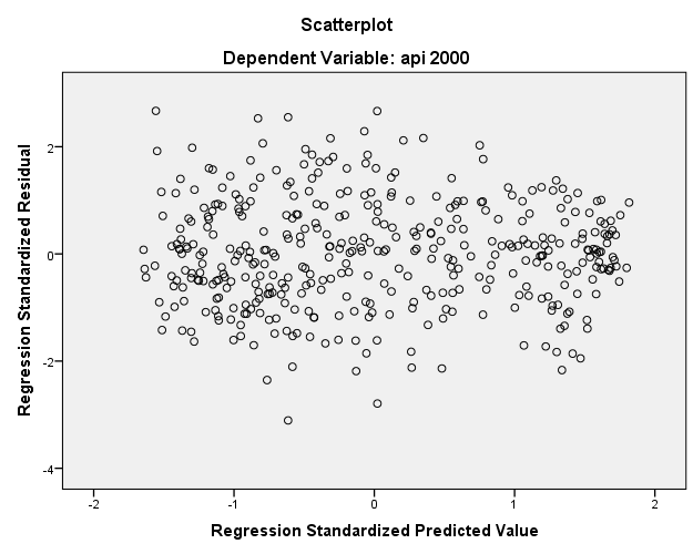
You can from this new residual that the trend is centered around zero but also that the variance around zero is scattered uniformly and randomly. We conclude that the linearity assumption is satisfied and the hetereoskedasticity assumption is satisfied if we run the fully specified predictive model. We will talk more about Model Specification in Section 2.3.
2.2 Tests on Normality of Residuals
In linear regression, a common misconception is that the outcome has to be normally distributed, but the assumption is actually that the residuals are normally distributed. It is important to meet this assumption for the p-values for the t-tests to be valid. Let’s go back and predict academic performance (api00) from percent enrollment (enroll). Note that the normality of residuals assessment is model dependent meaning that this can change if we add more predictors. SPSS automatically gives you what’s called a Normal probability plot (more specifically a P-P plot) if you click on Plots and under Standardized Residual Plots check the Normal probability plot box.
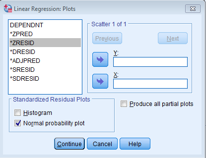
To create the more commonly used Q-Q plot in SPSS, you would need to save the standardized residuals as a variable in the dataset, in this case it will automatically be named ZRE_1. In Linear Regression click on Save and check Standardized under Residuals.
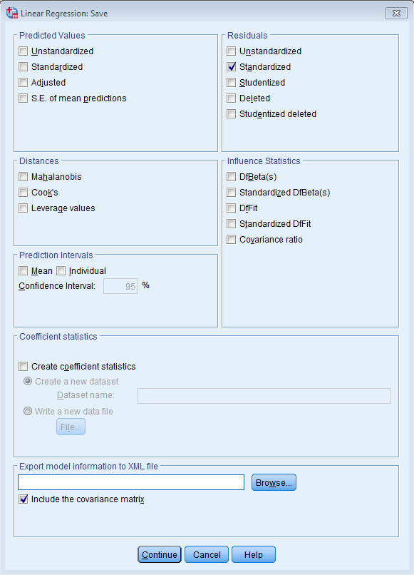
The code after pasting the dialog box will be:
	REGRESSION
	/MISSING LISTWISE
	/STATISTICS COEFF OUTS R ANOVA
	/CRITERIA=PIN(.05) POUT(.10)
	/NOORIGIN
	/DEPENDENT api00
	/METHOD=ENTER enroll
	/RESIDUALS NORMPROB(ZRESID)
	/SAVE ZRESID.
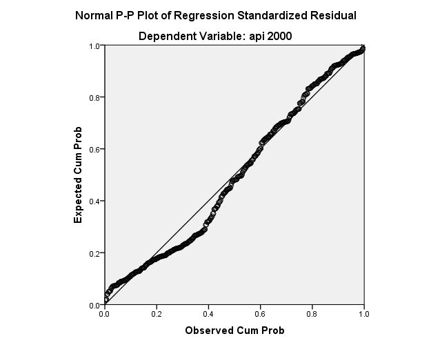
The plot is shown below. The P-P plot compares the observed cumulative distribution function (CDF) of the standardized residual to the expected CDF of the normal distribution. Note that we are testing the normality of the residuals and not predictors.
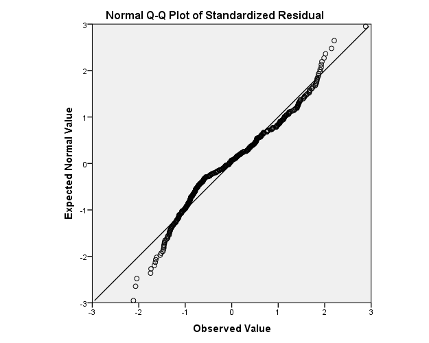
More commonly seen is the Q-Q plot, which compares the observed quantile with the theoretical quantile of a normal distribution. According to SAS Documentation Q-Q plots are better if you want to compare to a family of distributions that vary on location and scale; it is also more sensitive to tail distributions. Click on Analyze – Descriptive Statistics – Q-Q Plots.
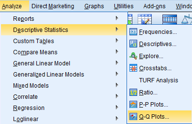
Then shift the newly created variable ZRE_1 to the Variables box and click Paste.

The code that we get from this is:
	PPLOT
	/VARIABLES=ZRE_1
	/NOLOG
	/NOSTANDARDIZE
	/TYPE=Q-Q
	/FRACTION=BLOM
	/TIES=MEAN
	/DIST=NORMAL.
The resulting Q-Q plot is show below. If the distribution is normal, then we should expect the points to cluster around the horizontal line. Note the difference in the tail distributions in the Q-Q plot versus the P-P plot above.
Before moving on to the next section, let’s first clear the ZRE_1 variable. Go to Variable View, right click on the Variable Number corresponding to ZRE_1 (in this case 25) and click Clear.

Alternatively you can use the following syntax to delete the ZRE_1 variable:
DELETE VARIABLES ZRE_1.
2.3 Model Specification
A model specification error can occur when one or more relevant variables are omitted from the model or one or more irrelevant variables are included in the model. If relevant variables are omitted from the model, the common variance they share with included variables may be wrongly attributed to those variables, and the error term can be inflated. On the other hand, if irrelevant variables are included in the model, the common variance they share with included variables may be wrongly attributed to them. Model specification errors can substantially affect the estimate of regression coefficients.
Consider the model below which is the same model we started with in Lesson 1 except that we take out meals as a predictor. This means we are only using full and acs_k3 as predictors of api00.
| Model | Unstandardized Coefficients | Standardized Coefficients | t | Sig. | |||
| B | Std. Error | Beta | |||||
| 1 | (Constant) | 32.213 | 84.075 | .383 | .702 | ||
| pct full credential | 5.390 | .396 | .564 | 13.598 | .000 | ||
| avg class size k-3 | 8.356 | 4.303 | .080 | 1.942 | .053 | ||
| a. Dependent Variable: api 2000 | |||||||
This regression model suggests that as class size increases academic performance increases, with p = 0.053 (which is marginally significant at alpha=0.05). More precisely, it says that for a one student increase in average class size, the predicted API score increases by 8.38 points holding the percent of full credential teachers constant. Before we publish results saying that increased class size is associated with higher academic performance, let’s check the model specification. We begin by asking to Save the Standardized Residuals.
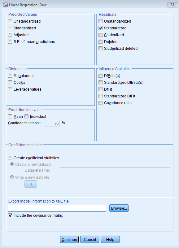
The syntax you obtain from checking the box is shown below:
	REGRESSION
	/MISSING LISTWISE
	/STATISTICS COEFF OUTS R ANOVA
	/CRITERIA=PIN(.05) POUT(.10)
	/NOORIGIN
	/DEPENDENT api00
	/METHOD=ENTER full acs_k3
	/SAVE ZRESID.
We see now in our dataset a new variable called ZRE_1. We can graph this variable (along the x-axis) with the percent of free meals on the y-axis. If in fact meals had no relationship with our model, it would be independent of the residuals.
	GRAPH
	/SCATTERPLOT(BIVAR)=meals WITH ZRE_1
	/MISSING=LISTWISE.
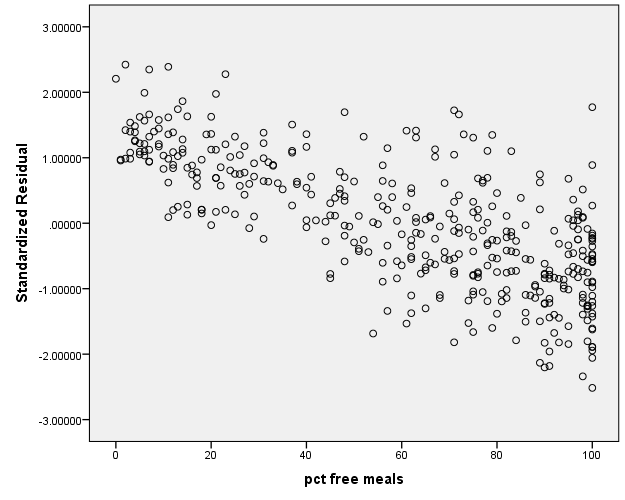
From the graph, we can see that percent free meals has a negative relationship with the residuals from our model using only average class size and percent full credential as predictors. Let’s take a look at the bivariate correlation among the three variables.
	CORRELATIONS
	/VARIABLES=api00 full acs_k3 meals
	/PRINT=TWOTAIL NOSIG
	/MISSING=PAIRWISE.
| api 2000 | pct full credential | avg class size k-3 | pct free meals | |||
| api 2000 | Pearson Correlation | 1 | .574** | .171** | -.901** | |
| Sig. (2-tailed) | .000 | .001 | .000 | |||
| N | 400 | 400 | 398 | 400 | ||
| pct full credential | Pearson Correlation | .574** | 1 | .161** | -.528** | |
| Sig. (2-tailed) | .000 | .001 | .000 | |||
| N | 400 | 400 | 398 | 400 | ||
| avg class size k-3 | Pearson Correlation | .171** | .161** | 1 | -.188** | |
| Sig. (2-tailed) | .001 | .001 | .000 | |||
| N | 398 | 398 | 398 | 398 | ||
| pct free meals | Pearson Correlation | -.901** | -.528** | -.188** | 1 | |
| Sig. (2-tailed) | .000 | .000 | .000 | |||
| N | 400 | 400 | 398 | 400 | ||
| **. Correlation is significant at the 0.01 level (2-tailed). |
||||||
From the correlation table you can see that meals and full are correlated with each other, but just as importantly they are both correlated with the outcome variable api00.
In fact, this satisifies two of the conditions of an omitted variable: that the omitted variable a) significantly predicts the outcome, and b) is correlated with other predictors in the model. Let’s re-run our regression model with the meals put back in. Note that this is the same model we began with in Lesson 1.
	REGRESSION
	/MISSING LISTWISE
	/STATISTICS COEFF OUTS R ANOVA
	/CRITERIA=PIN(.05) POUT(.10)
	/NOORIGIN
	/DEPENDENT api00
	/METHOD=ENTER full acs_k3 meals
	/SAVE ZRESID.
Since we saved the residuals a second time, SPSS automatically codes the next residual as ZRE_2. Now let’s plot meals again with ZRE_2.
	GRAPH
	/SCATTERPLOT(BIVAR)=meals WITH ZRE_2
	/MISSING=LISTWISE.
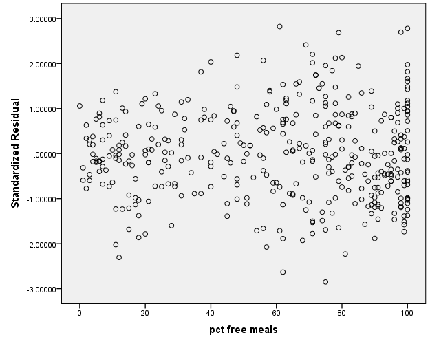
You can see that the previously strong negative relationship between meals and the standardized residuals is now basically flat. There seems to be some capping effect at meals = 100 but that may be due to the restricted range of the percentage. For more information about omitted variables, take a look at the StackExchange discussion forum.
2.4 Issues of Independence
The statement of this assumption is that the errors associated with one observation are not correlated with the errors of any other observation. Violation of this assumption can occur in a variety of situations. Consider the case of collecting data from our various school districts. It is likely that the schools within each school district will tend to be more like one another than schools from different districts, that is, their errors are not independent. From the saved standardized residuals from Section 2.3 (ZRE_1), let’s create boxplots of them clustered by district to see if there is a
pattern. Most notably, we want to see if the mean standardized residual is around zero for all districts and whether the variances are homogenous across districts.
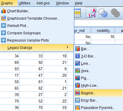
To explore these boxplots, go to Graphs – Legacy Dialogs – Boxplot.
Click on Simple – Data in Chart Are – Summaries for groups of cases – Define.
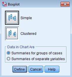
Under Define Simple Boxplot: Summaries for Groups of Cases select Variable:
ZRE_1, Category Axis: dnum, and Label Cases by: snum. Click Paste.

The syntax you obtain is shown below:
	EXAMINE VARIABLES=ZRE_1 BY dnum
	/PLOT=BOXPLOT
	/STATISTICS=NONE
	/NOTOTAL
	/ID=snum.
In particular, take a look at the boxplot produced from the Output.
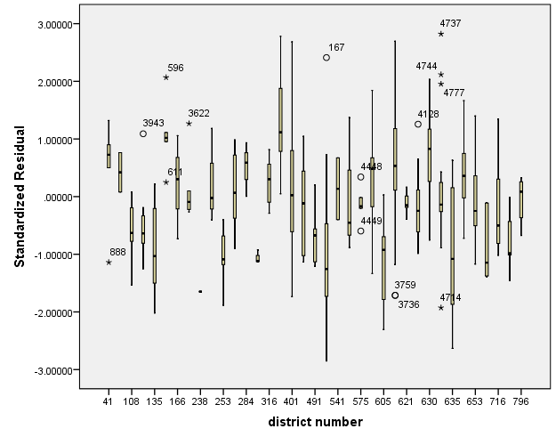
You can see that there is a possibility that districts tend to have different mean residuals not centered at zero. Additionally, some districts have more variability in residuals than other school districts. This suggests that the errors are not independent. Treatment of non-independent errors are beyond the scope of this seminar but there are many possible solutions.
2.5 Tests on Multicollinearity
When there is a perfect linear relationship among the predictors, the estimates for a regression model cannot be uniquely computed. The term collinearity implies that two variables are linear combinations of one another. When more than two variables are involved it is often called multicollinearity, although the two terms are often used interchangeably.
The primary concern is that as the degree of multicollinearity increases, the coefficient estimates become unstable and the standard errors for the coefficients can get wildly inflated. In this section, we will explore some SPSS commands that help to detect multicollinearity. Let’s proceed to the regression putting not_hsg, hsg, some_col, col_grad, and avg_ed as predictors of api00. Go to Linear Regression – Statistics and check Collinearity diagnostics.
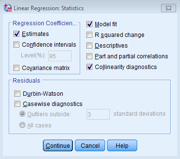
The syntax will populate COLLIN and TOL specifications values for the /STATISTICS subcommand. The TOL keyword tolerance is an indication of the percent of variance in the predictor that cannot be accounted for by the other predictors. This means that very small values indicate that a predictor is redundant, which means that values less than 0.10 are worrisome. The VIF, which stands for variance inflation factor, is (1/tolerance) and as a rule of thumb, a variable whose VIF values is greater than 10 are problematic. The syntax we obtain is shown below:
	REGRESSION
	/MISSING LISTWISE
	/STATISTICS COEFF OUTS R ANOVA COLLIN TOL
	/CRITERIA=PIN(.05) POUT(.10)
	/NOORIGIN
	/DEPENDENT api00
	/METHOD=ENTER not_hsg hsg some_col col_grad avg_ed.
| Model | Variables Entered | Variables Removed | Method |
| 1 | avg parent ed, parent some college, parent hsg, parent college grad, parent not hsgb |
. | Enter |
| a. Dependent Variable: api 2000 | |||
| b. Tolerance = .000 limit reached. | |||
| Model | Unstandardized Coefficients | Standardized Coefficients | t | Sig. | Collinearity Statistics |
||||
| B | Std. Error | Beta | Tolerance | VIF | |||||
| 1 | (Constant) | 867.555 | 1310.016 | .662 | .508 | ||||
| parent not hsg | -5.489 | 10.473 | -.793 | -.524 | .600 | .000 | 2434.887 | ||
| parent hsg | -3.652 | 7.846 | -.400 | -.465 | .642 | .001 | 786.223 | ||
| parent some college | -2.402 | 5.255 | -.180 | -.457 | .648 | .006 | 165.167 | ||
| parent college grad | -2.982 | 2.647 | -.340 | -1.127 | .261 | .010 | 96.749 | ||
| avg parent ed | 42.271 | 262.512 | .226 | .161 | .872 | .000 | 2099.164 | ||
| a. Dependent Variable: api 2000 | |||||||||
Note the high VIF values and extremely low tolerance values for avg_ed and not_hsg (and most of the other predictors). All of these variables measure parent’s education, and the very low tolerance values indicate that these variables contain redundant information. In this example, multicollinearity arises because we have put in too many variables that measure the same thing. Let’s check the bivariate correlations to see if we can find out a culprit.
	CORRELATIONS
	/VARIABLES=not_hsg hsg some_col col_grad avg_ed
	/PRINT=TWOTAIL NOSIG
	/MISSING=PAIRWISE.
| parent not hsg | parent hsg | parent some college | parent college grad | avg parent ed | ||
| parent not hsg | Pearson Correlation | 1 | .154** | -.357** | -.538** | -.852** |
| Sig. (2-tailed) | .002 | .000 | .000 | .000 | ||
| N | 400 | 400 | 400 | 400 | 381 | |
| parent hsg | Pearson Correlation | .154** | 1 | .057 | -.415** | -.551** |
| Sig. (2-tailed) | .002 | .258 | .000 | .000 | ||
| N | 400 | 400 | 400 | 400 | 381 | |
| parent some college | Pearson Correlation | -.357** | .057 | 1 | .155** | .303** |
| Sig. (2-tailed) | .000 | .258 | .002 | .000 | ||
| N | 400 | 400 | 400 | 400 | 381 | |
| parent college grad | Pearson Correlation | -.538** | -.415** | .155** | 1 | .809** |
| Sig. (2-tailed) | .000 | .000 | .002 | .000 | ||
| N | 400 | 400 | 400 | 400 | 381 | |
| avg parent ed | Pearson Correlation | -.852** | -.551** | .303** | .809** | 1 |
| Sig. (2-tailed) | .000 | .000 | .000 | .000 | ||
| N | 381 | 381 | 381 | 381 | 381 | |
| **. Correlation is significant at the 0.01 level (2-tailed). | ||||||
It looks like avg_ed is highly correlated with a lot of other variables. Let’s omit this variable and take a look at our analysis again.
	REGRESSION
	/MISSING LISTWISE
	/STATISTICS COEFF OUTS R ANOVA COLLIN TOL
	/CRITERIA=PIN(.05) POUT(.10)
	/NOORIGIN
	/DEPENDENT api00
	/METHOD=ENTER not_hsg hsg some_col col_grad.
The output you obtain from running the syntax above is:
| Model | Unstandardized Coefficients | Standardized Coefficients | t | Sig. | Collinearity Statistics |
||||
| B | Std. Error | Beta | Tolerance | VIF | |||||
| 1 | (Constant) | 745.625 | 19.899 | 37.471 | .000 | ||||
| parent not hsg | -3.876 | .294 | -.563 | -13.164 | .000 | .632 | 1.582 | ||
| parent hsg | -1.921 | .329 | -.221 | -5.840 | .000 | .811 | 1.233 | ||
| parent some college | .671 | .460 | .053 | 1.457 | .146 | .860 | 1.163 | ||
| parent college grad | 1.073 | .380 | .124 | 2.821 | .005 | .597 | 1.674 | ||
| a. Dependent Variable: api 2000 | |||||||||
Note that the VIF values in the analysis above appear much better. Also, note how the standard errors are reduced for the parent education variables. This is because the high degree of collinearity caused the standard errors to be inflated hence the term variance inflation factor. With the multicollinearity eliminated, the coefficient for most of the predictors, which had been non-significant, is now significant.
2.6 Unusual and Influential data
A single observation that is substantially different from all other observations can make a large difference in the results of your regression analysis. If a single observation (or small group of observations) substantially changes your results, you would want to know about this and investigate further. There are three ways that an observation can be unusual.
Outliers: In linear regression, an outlier is an observation with large residual. In other words, it is an observation whose dependent-variable value is unusual given its values on the predictor variables. An outlier may indicate a sample peculiarity or may indicate a data entry error or other problems.
Leverage: An observation with an extreme value on a predictor variable is called a point with high leverage. Leverage is a measure of how far an observation deviates from the mean of that variable. These leverage points can have an unusually large effect on the estimate of regression coefficients.
Influence: An observation is said to be influential if removing the observation substantially changes the estimate of coefficients. Influence can be thought of as the product of leverage and outlierness.
Recall that adding enroll into our predictive model seemed to be a problematic from the assumption checks we performed above. In order to visualize outliers, leverage and influence for this particular model descriptively, let’s make simple scatterplot of enroll and api00.
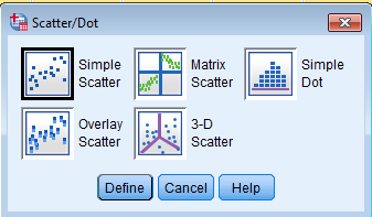
Go to Graphs – Legacy Dialogs – Scatter/Dot – Simple Scatter – Define.
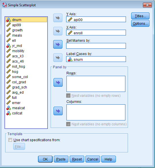
Move api00 to the Y Axis, and enroll to the X Axis, and Label Cases by: snum.
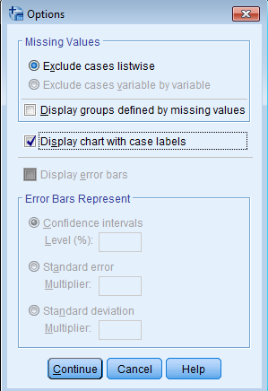
Within Simple Scatterplot, click on Options, and within this menu system, check Display chart with case labels. This will put the School Number next to the circular points so you can identify the school.
The syntax you obtain is as follows:
	GRAPH
	/SCATTERPLOT(BIVAR)=enroll WITH api00 BY snum (NAME)
	/MISSING=LISTWISE.
The scatterplot you obtain is shown below:
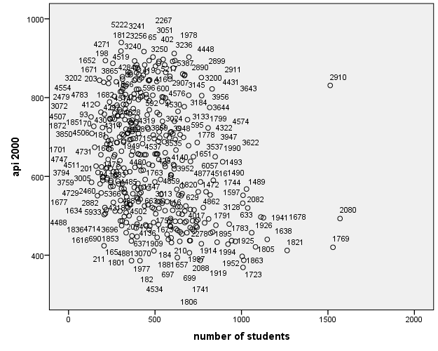
It seems like schools 2910, 2080 and 1769 are worth looking into because they stand out from all of the other schools. However it seems that School 2910 in particular may be an outlier, as well as have high leverage, indicating high influence. We will keep this in mind when we do our regression analysis. Let’s examine the standardized residuals as a first means for identifying outliers first using simple linear regression. From Analyze – Regression – Linear click on Plots and click Histogram under Standardized Residual Plots.
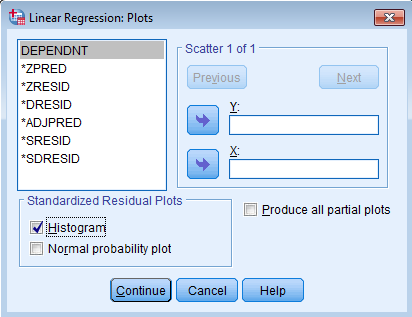
You will obtain a table of Residual Statistics. Note that the mean of an unstandardized residual should be zero (see Assumptions of Linear Regression), as should standardized value
| Minimum | Maximum | Mean | Std. Deviation | N | |
| Predicted Value | 430.46 | 718.27 | 647.62 | 45.260 | 400 |
| Residual | -285.500 | 389.148 | .000 | 134.857 | 400 |
| Std. Predicted Value | -4.798 | 1.561 | .000 | 1.000 | 400 |
| Std. Residual | -2.114 | 2.882 | .000 | .999 | 400 |
| a. Dependent Variable: api 2000 | |||||
You will get a table with Residual Statistics and a histogram of the standardized residual based on your model. Note that the unstandardized residuals have a mean of zero, and so do standardized predicted values and standardized residuals.
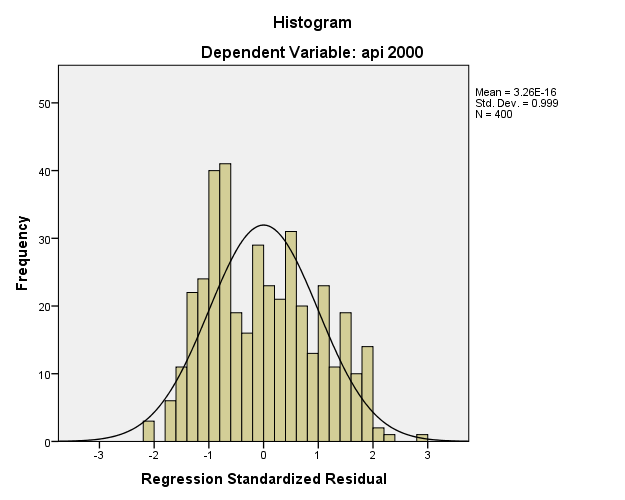
From the histogram you can see a couple of values at the tail ends of the distribution. If we paste the syntax, we will get something like:
	REGRESSION
	/MISSING LISTWISE
	/STATISTICS COEFF OUTS R ANOVA
	/CRITERIA=PIN(.05) POUT(.10)
	/NOORIGIN
	/DEPENDENT api00
	/METHOD=ENTER enroll
	/RESIDUALS HISTOGRAM(ZRESID).
Here’s where we need a little modification of the syntax (no more dialog boxes for now!). In addition to the histogram of the standardized residuals, we want to request the Top 10 cases for the standardized residuals, leverage and Cook’s D. Additionally, we want it to be labeled by the School ID (snum) and not the Case Number. The additional subcommands are shown below.
	REGRESSION
	/MISSING LISTWISE
	/STATISTICS COEFF OUTS R ANOVA
	/CRITERIA=PIN(.05) POUT(.10)
	/NOORIGIN
	/DEPENDENT api00
	/METHOD=ENTER enroll
	/RESIDUALS HISTOGRAM(ZRESID) OUTLIERS(ZRESID LEVER COOK) ID(snum).
The partial output you obtain is shown here:
| Case Number | school number | Statistic | Sig. F | ||
| Std. Residual | 1 | 8 | 2910 | 2.882 | |
| 2 | 242 | 4448 | 2.206 | ||
| 3 | 86 | 3236 | 2.147 | ||
| 4 | 192 | 1977 | -2.114 | ||
| 5 | 67 | 690 | -2.068 | ||
| 6 | 226 | 211 | -2.042 | ||
| 7 | 196 | 1978 | 2.019 | ||
| 8 | 339 | 5387 | 1.985 | ||
| 9 | 239 | 2267 | 1.941 | ||
| 10 | 11 | 2911 | 1.927 | ||
| Cook’s Distance | 1 | 8 | 2910 | .252 | .777 |
| 2 | 48 | 3643 | .014 | .986 | |
| 3 | 172 | 1723 | .014 | .986 | |
| 4 | 67 | 690 | .014 | .986 | |
| 5 | 11 | 2911 | .012 | .988 | |
| 6 | 242 | 4448 | .012 | .989 | |
| 7 | 140 | 1863 | .011 | .989 | |
| 8 | 193 | 1952 | .010 | .990 | |
| 9 | 19 | 3956 | .008 | .992 | |
| 10 | 47 | 3644 | .008 | .992 | |
| Centered Leverage Value | 1 | 210 | 2080 | .058 | |
| 2 | 163 | 1769 | .053 | ||
| 3 | 8 | 2910 | .052 | ||
| 4 | 120 | 1821 | .030 | ||
| 5 | 145 | 1638 | .022 | ||
| 6 | 164 | 1941 | .020 | ||
| 7 | 187 | 1678 | .019 | ||
| 8 | 197 | 1805 | .017 | ||
| 9 | 134 | 1926 | .016 | ||
| 10 | 130 | 2082 | .015 | ||
| a. Dependent Variable: api 2000 | |||||
You can see that School Number now appears as a column in the table above. This will save us time from having to go back and forth to the Data View. Case Number is the order in which the observation appears in the SPSS Data View; don’t confuse it with the School Number. Note that the Case Number may vary depending on how your data is sorted, but the School Number should be the same as the table above.
- standardized residuals: We are looking for values greater than 2 and less than -2 (outliers)
- leverage: a school with leverage greater than (2k+2)/n should be carefully examined. Here k is the number of predictors and n is the number of observations, so a value exceeding (2*1+2)/400 = 0.01 would be worthy of further investigation. School 2910 is one that has both a large standardized residual and leverage, which suggests that it may be influential.
- Cook’s Distance: Now let’s look at Cook’s Distance, which combines information on the residual and leverage. The lowest value that Cook’s D can assume is zero, and the higher the Cook’s D is, the more influential the point is. The conventional cut-off point is 4/n, or in this case 4/400 or .01. School 2910 is the top influential point.
- DFBETA: Cook’s Distance can be thought of as a general measure of influence. You can also consider more specific measures of influence that assess how each coefficient is changed by including the observation. Imagine that you compute the regression coefficients for the regression model with a particular case excluded, then recompute the model with the case included,
and you observe the change in the regression coefficients due to including that case in the model. This measure is called DFBETA and a DFBETA value can be computed for each observation for each predictor.
Let’s see which coefficient School 2910 has the most effect on. Since we only have a simple linear regression, we can only assess its effect on the intercept and enroll. Under Analyze – Linear Regression – Save – Influence Statistics, check DfBeta(s) and click Continue.
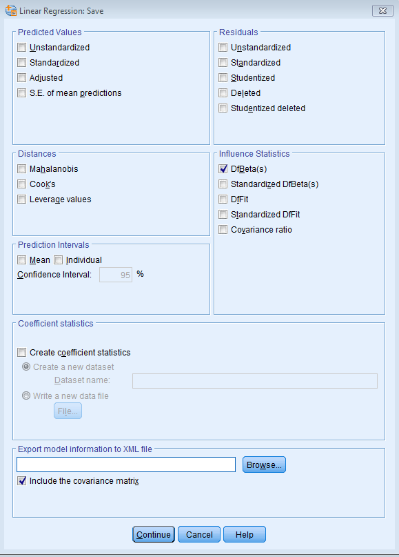
The code you obtain from pasting the syntax is shown below:
	REGRESSION
	/MISSING LISTWISE
	/STATISTICS COEFF OUTS R ANOVA
	/CRITERIA=PIN(.05) POUT(.10)
	/NOORIGIN
	/DEPENDENT api00
	/METHOD=ENTER enroll
	/SAVE DFBETA.
The newly created variables will appear in Data View. If you don’t specify a name, the variables will default to DFB0_1 and DFB1_1. Let’s juxtapose our api00 and enroll variables next to our newly created DFB0_1 and DFB1_1 variables in Variable View. Go back to Data View and right click on any space within DFB1_1 to click on Sort Descending. This will rank the highest DFBETAs on the enroll variable.
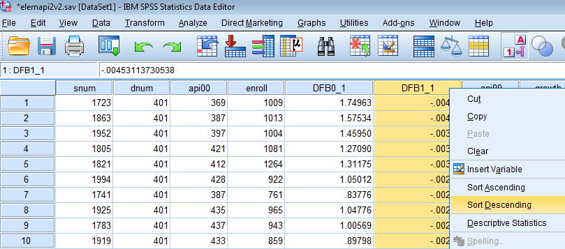
We can see below that School 2910 again pops up as a highly influential school not only for enroll but for our intercept as well. However, it does not pass our threshold of 0.1 for enroll.
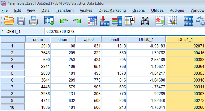
The table below summarizes the general rules of thumb we use for the measures we have discussed for identifying observations worthy of further investigation (where k is the number of predictors and n is the number of observations). What we see is that School 2910 passes the threshold for Leverage (.052), Standardized Residuals (2.882), and Cook’s D (0.252). Looking more specifically on the influence of School 2910 on particular parameters of our regression, DFBETA indicates that School 2910 has a large influence on our intercept term (causing a -8.98 estimated drop in api00 if this school were removed from the analysis). Although School 2910 does not pass the threshold for DFBETA on our enroll coefficient, if it were removed, it would show the largest change enroll among all the other schools. Finally, the visual description where we suspected Schools 2080 and 1769 as possible outliers does not pass muster after running these diagnostics. As a researcher then, we should investigate whether we should remove School 2910 from our analysis.
|
Measure |
Threshold | Value in this example |
| LEVER | > (2k+2)/n | 0.01 (for 1 predictor) 0.02 (for 3 predictors) |
| abs(ZRESID) | > 2 | 2 |
| Cook’s D | > 4/n | 0.01 |
| abs(SDBETA*) | > 2/sqrt(n) | 0.1 |
*Note that SDBETA is Standardized DFBETA and not DFBETA.
2.7 Summary
This chapter has covered a variety of topics in assessing the assumptions of regression using SPSS, and the consequences of violating these assumptions. As we have seen, it is not sufficient to simply run a regression analysis, but to verify that the assumptions have been met because coefficient estimates and standard errors can fluctuate wildly (e.g., from non-significant to significant after dropping avg_ed). If this verification stage is omitted and your data does not meet the assumptions of linear regression, your results could be misleading and your interpretation of your results could be in doubt. Without thoroughly checking your data for problems, it is possible that another researcher could analyze your data and uncover such problems and question your results showing an improved analysis that may contradict your results and undermine your conclusions.