- 3.0 Introduction
- 3.1 Regression with a 0/1 (dummy) variable
- 3.2 Regression with a 1/2 variable
- 3.3 Regression with a 1/2/3 (multicategory) variable
- 3.4 Regression with two categorical predictors (main effects model)
- 3.5 Regression with the interaction of two categorical predictors
- 3.6 Summary
- Go to Launch Page
3.0 Introduction
In the previous two lessons, we focused on regression analyses using Scale predictors. However, it is possible to include Nominal predictors in a regression analysis, but it requires some extra work in properly interpreting the results. Nominal and categorical variables are used interchangeably in this lesson. A regression with categorical predictors is possible because of what’s known as the General Linear Model (of which Analysis of Variance or ANOVA is also a part of). This lesson will show you how to perform regression with a dummy variable, a multicategory variable, multiple categorical predictors as well as the interaction between them. Other than Section 3.1 where we use the REGRESSION command in SPSS, we will be working with the General Linear Model (via the UNIANOVA command) in SPSS.
We will continue to use the elemapi2v2 data set we used in Lessons 1 and 2 of this seminar. Recall that the variable api00 is a measure of the school academic performance. The variable yr_rnd is a Nominal variable that is coded 0 if the school is not year round and 1 if year round. The variable meals is the percentage of students in the school who are receiving state sponsored free meals and can be used as a proxy for socioeconomic status. This was broken into 3 categories (to make equally sized groups) creating the variable mealcat.
Before we begin, we need to clarify what a dummy variable is (it’s actually rather smart!). Simply put, a dummy variable is a Nominal variable that can take on either 0 or 1. In your regression model, if you have k categories you would include only k-1 dummy variables in your regression because any one dummy variable is perfectly collinear with remaining set of dummies. For example, for the variable yr_rnd, if you know that the particular school is a Non-Year Round school (coded 0), you automatically know that it’s not a Year-Round school (coded 1). For mealcat, if you know that the school is not in the first and the second categories, it must be in the third category. This omitted variable is also known as the reference group because it is the group from which all other groups are compared.
The possible Dummy variables are listed down the rows and the variable categories are indicated in the columns for yr_rnd and mealcat. The reference category is highlighted in dark gray and omitted dummy variable is indicated by a row highlighted in green. We want to exclude dummy variables that have a ‘1’ value in any of the dark gray columns.Let’s look at how Year Round can be dummy coded:
| Year Round | Values | |
| Variable | Yes | No |
| Dummy1 | 1 | 0 |
| Dummy2 | 0 | 1 |
The reference group Dummy2 is highlighted in green. It is also the dummy code indicating Not Year Round. The Meal Categories are dummy coded as shown here:
| Meal Category | Values | ||
| Variable | First | Second | Third |
| Dummy1 | 1 | 0 | 0 |
| Dummy2 | 0 | 1 | 0 |
| Dummy3 | 0 | 0 | 1 |
The reference group here is Dummy3, it is also the dummy variable indicating the third meal category. For additional information on dummy coding, take a look at Section 4.1.1 in our page SAS Seminar: Analyzing and Visualizing Interactions.
3.1 Regression with a 0/1 (dummy) variable
Now that we are familiar with dummy coding, let’s put them into our regression model. The most fundamental method of incorporating a Nominal predictor in a regression analysis is by using a dummy variable. Let’s use the variable yr_rnd as an example of a dummy variable. Here yr_rnd is a predictor of api00. We suspect that Year Round schools will perform better than Not Year Round schools. Go to Analyze – Regression – Linear. Shift api00 into Dependent and yr_rnd into Independent(s).
The code you obtain from pasting the syntax is:
	DATASET ACTIVATE DataSet1.
	REGRESSION
	/MISSING LISTWISE
	/STATISTICS COEFF OUTS R ANOVA
	/CRITERIA=PIN(.05) POUT(.10)
	/NOORIGIN
	/DEPENDENT api00
	/METHOD=ENTER yr_rnd.
This is essentially the same code as we used in Lesson 1 except that now instead of a Scale predictor we are including a Nominal dummy variable. The output is shown below. Let’s exclude the Model Summary and ANOVA tables for now and concentrate on the Coefficients.
| Model | Unstandardized Coefficients | Standardized Coefficients | t | Sig. | ||
| B | Std. Error | Beta | ||||
| 1 | (Constant) | 684.539 | 7.140 | 95.878 | .000 | |
| year round school | -160.506 | 14.887 | -.475 | -10.782 | .000 | |
| a. Dependent Variable: api 2000 | ||||||
This may seem odd at first, but this is a legitimate analysis. But what does this mean? Let’s go back to basics and write out the regression equation that this model implies.
$$\hat{\mbox{API00}} =\hat{b}_0 + \hat{b}_1*(\mbox{YR_RND})$$
where \(\hat{b}_0\) is the estimated intercept and \(\hat{b}_1\) is the estimated coefficient for variable yr_rnd. Filling in the values from the regression equation, we get
$$ \hat{\mbox{API00}} = 684.54 – 160.51*(\mbox{YR_RND})$$
If a school is not a year-round school (i.e., yr_rnd is 0) the regression equation would simplify to:
$$\begin{align} \hat{\mbox{API00}} & = 684.54 – 160.51*(\mbox{YR_RND=0}) \\ & = 684.54 – 0 \\ & = 684.54 \end{align}$$
This means that the intercept you obtain from the regression coefficient is the mean predicted API score for non-year round schools.
If a school is a year-round school, the regression equation would simplify to:
$$\begin{align} \hat{\mbox{API00}} & = 684.54 – 160.51*(\mbox{YR_RND=1}) \\ & = 684.54 – 160.51 \\ & = 524.03 \end{align}$$
(Optional)Plotting the regression coefficient
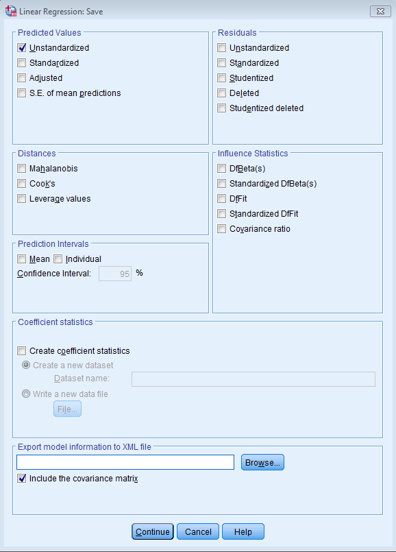
Let’s take a look at this graphically. In order to do so we can plot the predicted values against yr_rnd2 by first saving the unstandardized predicted values. Under Linear Regression click on Save, check the Unstandardized box in the Predicted Values field.
The syntax you obtain is as follows:
	REGRESSION
	/MISSING LISTWISE
	/STATISTICS COEFF OUTS R ANOVA
	/CRITERIA=PIN(.05) POUT(.10)
	/NOORIGIN
	/DEPENDENT api00
	/METHOD=ENTER yr_rnd
	/SAVE PRED.
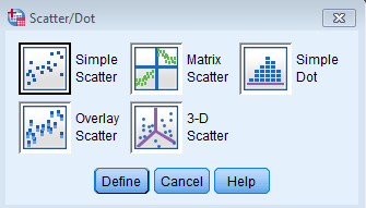
After you run the syntax, you should get a new variable in your dataset called PRE_1. What we want is to plot PRE_1 (the unstandardized predicted values) on the y-axis (the vertical axis) and yr_rnd on the x-axis (horizontal axis). To do so we can use a simple scatterplot. Go to Graphs – Legacy Dialogs – Scatter/Dot – Simple Scatter.
Shift PRE_1 to the Y-axis field and yr_rnd in the X-axis field.
The code you obtain from pasting the syntax is:
	GRAPH
	/SCATTERPLOT(BIVAR)=yr_rnd WITH PRE_1
	/MISSING=LISTWISE.
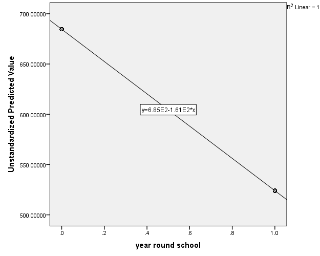
It looks like two points but in fact there are many predicted points overlayed on top of each other, 308 points for non-year round schools and 92 points for year round schools (you can confirm this by splitting the file by going to Data – Split File – Organize output by groups – Groups based on: yr_rnd and then going to Analyze – Descriptive Statistics – Descriptives – Variables: api00). This is because we only performed a simple linear regression such that all schools in year round schools got one value and all schools in non-year round schools got another value. To see the linear trend, double click on Add Trendline, you can see that y=6.85E2-1.61E2*x which is scientific notation for y=685-161*x, where E2 means multiply by 100.
From the plot below it appears that yr_rnd is a continuous variable, but that’s essentially how the “hack” works, the linear regression is still thinking yr_rnd is a continuous variable, but one that can only take on two values, 0 and 1. Note the technique was modeled off of this site.
Although yr_rnd only has two values, 0 and 1, we can still draw a regression line showing the relationship between yr_rnd and api00. Based on the results above, we see that the predicted value for non-year round schools is 684.539 and the predicted value for the year round schools is 524.032, and the slope of the line is negative, which makes sense since the coefficient for yr_rnd was negative (-160.5064).
Let’s relate these predicted values back to the regression equation. For the non year-round schools, their predicted api00 score is the intercept (684.539). The coefficient for yr_rnd is the amount we need to add to get the mean for the year-round schools, i.e., we need to add -160.5064 to get 524.0326, which is the mean for the year-round schools. In other words, the coefficient for yr_rnd is the difference of predicted api00 scores for year round versus non-year round schools.
Same analysis with an Independent T Test
It may be surprising to note that this regression analysis with a single dummy variable is the same as doing an independent t-test comparing the mean api00 for the year-round schools with the non year-round schools (see below). You can see that the t-value below is the same as the t-value for yr_rnd in the regression above.
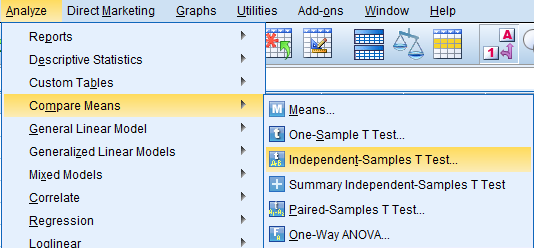
Go to Analyze – Compare Means – Independent Samples T Test:
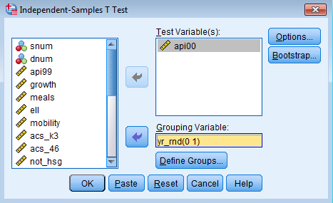
Move api00 over to the Test Variable(s) field and yr_rnd in the Grouping Variable field:
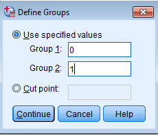
In SPSS, you need to define groups in an independent t-test until you no longer see yr_rnd(? ?) under the Grouping Variable field. Click on Define Groups…
Here we define Group 1 to be 0, which defines the non-year round schools and Group 2 is 1 which defines the year-round schools. See how the question marks disappear:
The code you obtain from pasting the syntax is:
	T-TEST GROUPS=yr_rnd(0 1)
	/MISSING=ANALYSIS
	/VARIABLES=api00
	/CRITERIA=CI(.95).
The output you obtain from running the syntax is as follows:
| year round school | N | Mean | Std. Deviation | Std. Error Mean | |
| api 2000 | No | 308 | 684.54 | 132.113 | 7.528 |
| Yes | 92 | 524.03 | 98.916 | 10.313 | |
| Levene’s Test for Equality of Variances | t-test for Equality of Means | |||||||||
| F | Sig. | t | df | Sig. (2-tailed) | Mean Difference | Std. Error Difference | 95% Confidence Interval of the Difference | |||
| Lower | Upper | |||||||||
| api 2000 | Equal variances assumed | 20.539 | .000 | 10.782 | 398 | .000 | 160.506 | 14.887 | 131.239 | 189.774 |
| Equal variances not assumed | 12.571 | 197.215 | .000 | 160.506 | 12.768 | 135.327 | 185.686 | |||
You can see that the Mean Difference of 160.506 is exactly the same as the coefficient in the simple linear regression except that the sign is reversed. This can easily be changed if we define Group 1 to be year round schools and Group 2 to be non-year round schools.
Same analysis with Univariate ANOVA
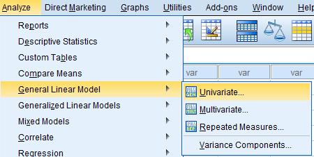
Additionally, the t-statistic squared is the F statistic for an independent t-test, hence we can run a One-Way ANOVA with two groups. Go to Analyze – General Linear Model – Univariate.
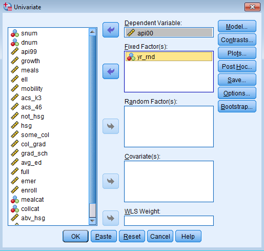
Move api00 to the Dependent Variable field and yr_rnd to the Fixed Factor field.
The code we obtain is:
	UNIANOVA api00 BY yr_rnd
	/METHOD=SSTYPE(3)
	/INTERCEPT=INCLUDE
	/CRITERIA=ALPHA(0.05)
	/DESIGN=yr_rnd.
In SPSS, a variable after the BY keyword is a Fixed Factor (or categorical variable) and a variable after the WITH statement is a Covariate (or a continuous variable). Here we are only interested in Fixed Factors. The output we obtain from running the code is:
| Value Label | N | ||
| year round school | 0 | No | 308 |
| 1 | Yes | 92 | |
|
||||||
| Source | Type III Sum of Squares | df | Mean Square | F | Sig. | |
| Corrected Model | 1825000.563a | 1 | 1825000.563 | 116.241 | .000 | |
| Intercept | 103472108.743 | 1 | 103472108.743 | 6590.505 | .000 | |
| yr_rnd | 1825000.563 | 1 | 1825000.563 | 116.241 | .000 | |
| Error | 6248671.435 | 398 | 15700.179 | |||
| Total | 175839633.000 | 400 | ||||
| Corrected Total | 8073671.997 | 399 | ||||
| a. R Squared = .226 (Adjusted R Squared = .224) | ||||||
If you square the t-value, (10.782)*(10.782) = 116.252, it matches the F statistic from the Univariate ANOVA table above (minus rounding error), showing another way in which the t-test is the same as the ANOVA test.
3.2: Regression with a 1/2 variable
From the previous section we know that a regression coefficient with a categorical variable is that same as a t-test. Additionally, recall that if you square the t-value, you will get the F-value: 10.782*10.782 = 116.25 (give and take rounding error). This implies that a regression with categorical predictors is essentially the same as an ANOVA. In Section 3.1 however, we only showed you the ANOVA table. We will show how to reproduce the regression coefficients as well. Under General Linear Model – Univariate click Options and check the box for Parameter Estimates under the Display field.
The code you obtain is as follows. Note the additional subcommand and keyword /PRINT=PARAMETER.
	UNIANOVA api00 BY yr_rnd
	/METHOD=SSTYPE(3)
	/INTERCEPT=INCLUDE
	/PRINT=PARAMETER
	/CRITERIA=ALPHA(.05)
	/DESIGN=yr_rnd.
Now we can get the regression coefficients as shown below:
|
|||||||
| Parameter | B | Std. Error | t | Sig. | 95% Confidence Interval | ||
| Lower Bound | Upper Bound | ||||||
| Intercept | 524.033 | 13.063 | 40.114 | .000 | 498.351 | 549.715 | |
| [yr_rnd=0] | 160.506 | 14.887 | 10.782 | .000 | 131.239 | 189.774 | |
| [yr_rnd=1] | 0a | . | . | . | . | . | |
| a. This parameter is set to zero because it is redundant. | |||||||
Let’s first understand what SPSS is doing under the hood. When we put in yr_rnd as a Fixed Factor in SPSS Univariate ANOVA, SPSS will convert each level of the Nominal variable into a corresponding dummy variable. By default, SPSS assigns the reference group to be the level with the highest numerical value. In this case, yr_rnd = 1 is the highest value, which means Dummy1 is Non Year Round and Dummy2 is Year Round. Since Dummy2 is the reference group it is excluded from the analysis, hence the B = 0. The Intercept is the predicted api00 of the reference group, so it is the predicted api00 for Year Round schools. The dummy code table looks like this (note it’s reversed from our first table):
| Year Round | Values | |
| Variable | No | Yes |
| Dummy1 | 1 | 0 |
| Dummy2 | 0 | 1 |
In this case, SPSS is automatically assigning the Year Round Schools to Dummy2, but we actually want it to be Dummy1. In order to do this, and to replicate the B coefficients from Section 3.1 exactly, we need the reference group to be the Non Year-Round schools. In order to do this we need to do some recoding of yr_rnd. Go to Transform – Recode into Different Variables.
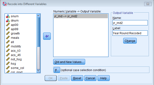
Under Output Variable assign Name to be yr_rnd2 and Label “Year Round Recoded” and click Change. You will see the new variable updated under Numeric Value -> Output Variable
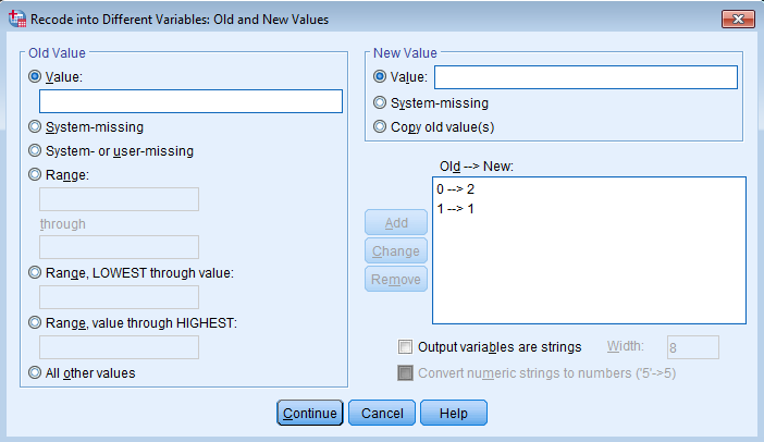
Click on Old and New Values… Under Old Value – Value enter 0 and New Value – Value enter 2. This makes Non-Year Round schools the highest numeric value which becomes the reference group in SPSS. Additionally, put another entry where Old Value – Value is 1 and New Value – Value is also 1. This will maintain the same coding for Year-Round schools. Click Continue and Paste.
The syntax you obtain from pasting the syntax above is:
	RECODE yr_rnd (0=2) (1=1) INTO yr_rnd2.
	VARIABLE LABELS yr_rnd2 'Year Round Recoded'.
	EXECUTE.
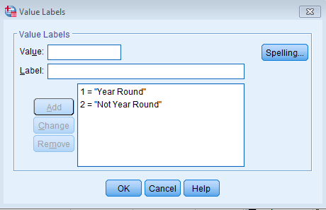
Additionally, in Variable View let’s create Value Labels for yr_rnd2 so we don’t confuse what the reference group is.
Let’s re-run the linear regression as a General Linear Model (using the SPSS command UNIANOVA) with the yr_rnd2 as the Fixed Factor.
 	UNIANOVA api00 BY yr_rnd2
	/METHOD=SSTYPE(3)
	/INTERCEPT=INCLUDE
	/PRINT=PARAMETER
	/CRITERIA=ALPHA(.05)
	/DESIGN=yr_rnd2.
The output you obtain from running the syntax is as follows:
|
|||||||
| Parameter | B | Std. Error | t | Sig. | 95% Confidence Interval | ||
| Lower Bound | Upper Bound | ||||||
| Intercept | 684.539 | 7.140 | 95.878 | .000 | 670.503 | 698.575 | |
| [yr_rnd2=1] | -160.506 | 14.887 | -10.782 | .000 | -189.774 | -131.239 | |
| [yr_rnd2=2] | 0a | . | . | . | . | . | |
| a. This parameter is set to zero because it is redundant. | |||||||
You can see now that the output you get is exactly the same as the regression with a 0/1 variable in Section 3.1, the Intercept is 684.539 and the B=-160.506.
3.3 Regression with a 1/2/3 (multicategory) variable
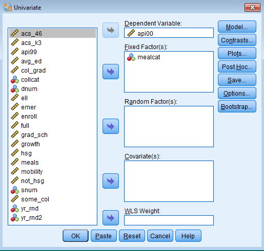
Regression with a multicategory (more than two levels) variable is basically an extension of regression with a 0/1 (a.k.a. dummy coded) or 1/2 variable. Instead of one dummy code however, think of k categories having k-1 dummy variables. For example if you have three categories, we will expect two dummy variables. Each dummy variable is then the difference between the category itself with the reference group. As we stated before, SPSS chooses the highest value as the reference group. Since we have three meal categories in mealcat, for example, the third meal category is now the reference group. Let’s go back and substitute in mealcat into the Fixed Factor(s) field for our Univariate General Linear Model (i.e., command UNIANOVA).
Go to Analyze – General Linear Model – Univariate.
The output you obtain is shown below:
| Value Label | N | ||
| Percentage free meals in 3 categories | 1 | 0-46% free meals | 131 |
| 2 | 47-80% free meals | 132 | |
| 3 | 81-100% free meals | 137 | |
|
||||||
| Source | Type III Sum of Squares | df | Mean Square | F | Sig. | |
| Corrected Model | 6094197.670a | 2 | 3047098.835 | 611.121 | .000 | |
| Intercept | 168847142.059 | 1 | 168847142.059 | 33863.695 | .000 | |
| mealcat | 6094197.670 | 2 | 3047098.835 | 611.121 | .000 | |
| Error | 1979474.328 | 397 | 4986.081 | |||
| Total | 175839633.000 | 400 | ||||
| Corrected Total | 8073671.998 | 399 | ||||
| a. R Squared = .755 (Adjusted R Squared = .754) | ||||||
|
|||||||
| Parameter | B | Std. Error | t | Sig. | 95% Confidence Interval | ||
| Lower Bound | Upper Bound | ||||||
| Intercept | 504.380 | 6.033 | 83.606 | .000 | 492.519 | 516.240 | |
| [mealcat=1] | 301.338 | 8.629 | 34.922 | .000 | 284.374 | 318.302 | |
| [mealcat=2] | 135.014 | 8.612 | 15.677 | .000 | 118.083 | 151.945 | |
| [mealcat=3] | 0a | . | . | . | . | . | |
| a. This parameter is set to zero because it is redundant. | |||||||
From the Between-Subjects Factors table we confirm that mealcat has three categories 0-46%, 47-80%, 81-100% free meals (the higher the percent, the lower the socioeconomic status). SPSS treats Fixed Factor(s) as Between Subjects Effects. Looking at the Tests of Between-Subjects Effects, the Model is significant. The row Corrected Model means that Type III Sum of Squares were used (we won’t cover that in this seminar, but it has something to do with unbalanced data since the sample size in each category is different). The important row to look at is the mealcat F(2,397) = 611.121. It is significant at alpha = 0.05, which implies that the predicted api00 scores of each of the three categories are not equal to each other.
The Parameter Estimates table tell us the differences in the predicted scores from the respective category to the reference category. The term [mealcat=1] is the additional increase in predicted api00 scores for the first category compared to the third category. Similarly, the term [mealcat=2] is the additional increase in predicted api00 scores for the second category compared to the third category. This makes sense given that we expect higher api00 scores for lower percent free meals at the school.
The Intercept is 504.380 which is the predicted api00 score of the reference group, [mealcat=3]. To obtain the predicted api00 score for the other two categories, we simply add the corresponding coefficient. For example, the predicted api00 score of [mealcat=1] is 504.380 + 301.338 = 805.718; the predicted api00 score of [mealcat=2] is 504.380 + 135.014 = 639.394. The reason that the coefficient (B) of [mealcat=3] is 0 is because it is the reference group, or you can say that the deviation from the Intercept is 0. To get the estimated means without calculating it ourselves, we can tell SPSS to give us the /EMMEANS.
(Optional) Getting estimated marginal means
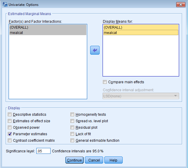
Under General Liner Model – Univariate, click on Options. Move the (OVERALL) and mealcat variables from the Factor(s) and Factor Interactions field to the Display Means for field and click Continue.
The code you obtain is shown below:
	UNIANOVA api00 BY mealcat
	/METHOD=SSTYPE(3)
	/INTERCEPT=INCLUDE
	/EMMEANS=TABLES(OVERALL)
	/EMMEANS=TABLES(mealcat)
	/PRINT=PARAMETER
	/CRITERIA=ALPHA(.05)
	/DESIGN=mealcat.
The addtional output table you obtain is shown:
|
||||
| Mean | Std. Error | 95% Confidence Interval | ||
| Lower Bound | Upper Bound | |||
| 649.830 | 3.531 | 642.888 | 656.773 | |
|
|||||
| Percentage free meals in 3 categories | Mean | Std. Error | 95% Confidence Interval | ||
| Lower Bound | Upper Bound | ||||
| 0-46% free meals | 805.718 | 6.169 | 793.589 | 817.846 | |
| 47-80% free meals | 639.394 | 6.146 | 627.311 | 651.477 | |
| 81-100% free meals | 504.380 | 6.033 | 492.519 | 516.240 | |
Note that the means you obtain from the 2. Percentage free meals in 3 categories table matches what we calculated manually. The 1. Grand Mean table does not match the Intercept term from the Parameter Estimates table because that term is reserved for the predicted score for api00 of the reference category, [mealcat=3]. To calculate the grand mean, simply average the predicted scores for each of the three mealcat categories, (805.718 + 639.394 + 504.380)/3= (1949.492)/3 = 649.83.
3.4 Regression with two categorical predictors (main effects model)
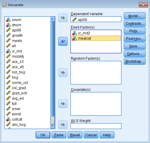
Suppose we want to know: What’s the effect of Year Round schools on academic performance, controlling for socioeconomic status? What if I thought that the effect of year round schools doesn’t change by the SES of the school? We can include both yr_rnd2 and mealcat together in the same model to test this out. Without an interaction between Year Round and Percent Free Meals, this is what’s called a main effects model. In order to start fitting our new model, recall that we want yr_rnd2 instead of yr_rnd when we are using the UNIANOVA command because SPSS takes the highest value and sets it to the reference group. In this case, we want the reference group to be non-year round schools. Let’s run the analysis first via the menu system. Go to Analyze – General Linear Model – Univariate and under Dependent Variable place api00 and under Fixed Factor(s) add in yr_rnd2 and mealcat.
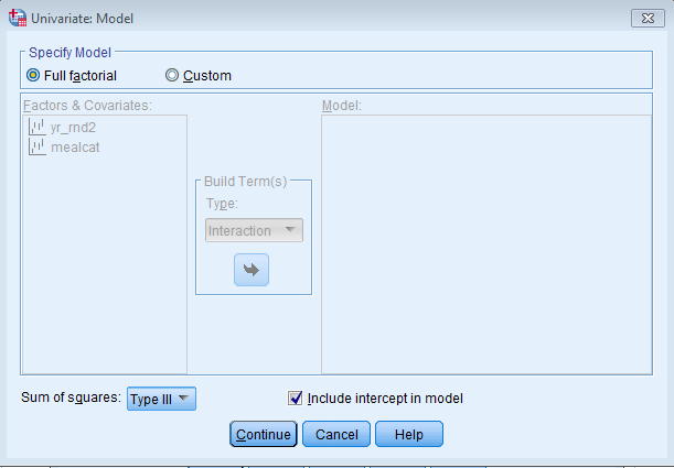
By default SPSS will interact Factor Variables in UNIANOVA. Since we only want the main effects, under the Specify Model field, click on Custom. Then under Build Terms – Type, select Main effects from the drop down menu. Shift yr_rnd2 and mealcat over from Factors & Covariates to Model.
Alternatively we can simply adjust the previous syntax by adding mealcat after the BY statement and also as a specification in the /DESIGN subcommand.
	UNIANOVA api00 BY yr_rnd2 mealcat
	/METHOD=SSTYPE(3)
	/INTERCEPT=INCLUDE
	/PRINT=PARAMETER
	/CRITERIA=ALPHA(.05)
	/DESIGN=yr_rnd2 mealcat.
The selected output we obtain from running the syntax is as follows:
|
||||||
| Source | Type III Sum of Squares | df | Mean Square | F | Sig. | |
| Corrected Model | 6194144.303a | 3 | 2064714.768 | 435.017 | .000 | |
| Intercept | 104733334.071 | 1 | 104733334.071 | 22066.395 | .000 | |
| yr_rnd2 | 99946.633 | 1 | 99946.633 | 21.058 | .000 | |
| mealcat | 4369143.740 | 2 | 2184571.870 | 460.270 | .000 | |
| Error | 1879527.694 | 396 | 4746.282 | |||
| Total | 175839633.000 | 400 | ||||
| Corrected Total | 8073671.997 | 399 | ||||
| a. R Squared = .767 (Adjusted R Squared = .765) | ||||||
Looking at the in the Tests of Between-Subjects Effects under the F and Sig columns, we see that the overall effect of yr_rnd2 and mealcat is significant. This tests within each Factor (or Nominal variable), whether the means of each level within each Factor are equal to each other. Suppose we want to get comparisons between particular levels of each of the categories, we need to look at the Parameter Estimates table. Before we do so, let’s first consider how these variables are dummy coded.
| Values | ||||||
| Year Round | Meal Category | |||||
| Dummy | Yes | No | First | Second | Third | |
| Year Round | Dummy1 | 1 | 0 | |||
| Dummy2 | 0 | 1 | ||||
| Meal Category | Dummy3 | 1 | 0 | 0 | ||
| Dummy4 | 0 | 1 | 0 | |||
| Dummy5 | 0 | 0 | 1 | |||
From this table we can see that there are a total of five dummy variables, 2 dummies for Year Round and Not Year Round, and 3 dummies for each of the three meal categories. The variables Dummy2 (Not Year Round) and Dummy5 (Third Meal Category) are redundant and hence excluded from our model. Additionally, these are the reference groups for Year Round and Meal Category. By putting both variables in our Factor list, SPSS is internally creating five dummy variables for us and purposely excluding Dummy2 and Dummy5 (green highlights).
|
|||||||
| Parameter | B | Std. Error | t | Sig. | 95% Confidence Interval | ||
| Lower Bound | Upper Bound | ||||||
| Intercept | 526.330 | 7.585 | 69.395 | .000 | 511.419 | 541.241 | |
| [yr_rnd2=1] | -42.960 | 9.362 | -4.589 | .000 | -61.365 | -24.555 | |
| [yr_rnd2=2] | 0a | . | . | . | . | . | |
| [mealcat=1] | 281.683 | 9.446 | 29.821 | .000 | 263.113 | 300.253 | |
| [mealcat=2] | 117.946 | 9.189 | 12.836 | .000 | 99.881 | 136.011 | |
| [mealcat=3] | 0a | . | . | . | . | . | |
| a. This parameter is set to zero because it is redundant. | |||||||
Because this model has only main effects (no interactions) you can interpret [yr_rnd2=1] as the difference between the year round and non-year round schools (year round schools have a lower predicted api00 holding mealcat constant). The coefficient for [mealcat=1] is the difference in predicted api00 between the first and third meal categories, and [mealcat=2] is the difference in predicted api00 between the second and third meal categories holding yr_rnd2 constant.
Interpreting Coefficients and Calculating Predicted Values
Let’s dig below the surface and see how the coefficients relate to the predicted values. In order to do this, we would have to know cell means which are mean api00 scores formed by crossing yr_rnd2 and mealcat. In the table below, we label each cell mean from c1 to c6.
| Meal Cat 1 | Meal Cat 2 | Meal Cat 3 | |
| Year Round | c1 | c2 | c3 |
| Non Year Round | c4 | c5 | c6 |
With respect to mealcat, the category third meal category is the reference category, and with respect to yr_rnd2 the second category or Non Year Round schools is the reference category. As a result, c6 (the sixth cell) is the reference cell. The Intercept term (highlighted in yellow) under the Parameter Estimates table is the predicted api00 for schools in the third highest percent free meal category and that are not year-round.
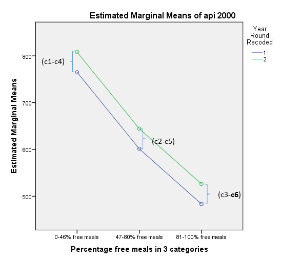
The coefficient for [yr_rnd2=1] is the difference between c3 and c6. In words, this means that the coefficient represents the Year Round effect on the predicted score of api00 for schools with a meal category of 3. Those in year round schools have a predicted api00 score that is 42.96 points lower than those not in year round schools. Since this is a main effects model, it is also the difference between c2 and c5, or from c1 and c4. This means that the difference in predicted api00 scores between year round and non-year round schools stays the same regardless of which meal category the school is in. These differences are the amount you add to the predicted value when you go from non-year round to year round schools above and beyond the effect of mealcat.
The coefficient for [mealcat=1] is the predicted difference between c4 and c6. It is the difference in the predicted api00 score between the first meal category and the third meal category for Non Year Round schools (the reference category). Since this model only has main effects, it is also the predicted difference between c1 and c3, which means that the predicted difference of api00 scores between the first meal category and the third meal category is the same for both year round and non-year round schools (note that this may or may not be true but it’s what we specify in the model). Likewise, [mealcat=2] is the predicted difference between c5 and c6, and also the predicted difference between c2 and c3. The coefficients of mealcat are the difference between the said category with the third category (reference group) holding yr_rnd2 constant (or regardless of the values of yr_rnd2). Collectively these are known as the main effects.
Let’s create a cross table of cell mean differences to clarify this further.
| Year Round | ||||
| Meal Cat 1 | Meal Cat 2 | Meal Cat 3 | ||
| Non Year Round | Meal Cat 1 | -42.96 | ||
| (c1-c4) | ||||
| Meal Cat 2 | -42.96 | |||
| (c1-c4)-(c2-c5) | (c2-c5) | |||
| Meal Cat 3 | -42.96 | |||
| (c1-c4)-(c3-c6) | (c2-c5)-(c3-c6) | (c3-c6) | ||
The blue cell is the simple effect of yr_rnd2 for Non Year Round schools which is (c3-6).
The gray boxes are cell mean differences that were omitted for simplicity. Since this is a main effects model, all difference of differences will be 0 (note this is not true for the interaction model).
Now that we know that the coefficients represent deviations from the reference cell, we can calculate the predicted api00 scores. In terms of the coefficients, they would be:
| Meal Cat 1 | Meal Cat 2 | Meal Cat 3 | |
| Year Round | Intercept | Intercept | Intercept |
| + [yr_rnd2=1] | + [yr_rnd2=1] | + [yr_rnd2=1] | |
| + [mealcat=1] | + [mealcat=2] | ||
| 765.053 | 601.316 | 483.37 | |
| c1 | c2 | c3 | |
| Non Year Round | Intercept | Intercept | Intercept |
| + [mealcat=1] | + [mealcat=2] | ||
| 808.013 | 644.276 | 526.33 | |
| c4 | c5 | c6 |
Note that the yellow term is the intercept we obtain from the Parameter Estimates table.
(Optional)Getting marginal means
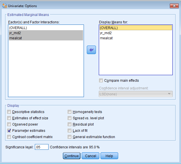
We can ask SPSS to output the means but they are the marginal means. Go to Analyze – General Linear Model – Univariate – Options. Move the (OVERALL), yr_rnd2 and mealcat variables from the Factor(s) and Factor Interactions field to the Display Means for field and click Continue.
The syntax you obtain is as follows:
	UNIANOVA api00 BY yr_rnd2 mealcat
	/METHOD=SSTYPE(3)
	/INTERCEPT=INCLUDE
	/EMMEANS=TABLES(OVERALL)
	/EMMEANS=TABLES(yr_rnd2)
	/EMMEANS=TABLES(mealcat)
	/PRINT=PARAMETER
	/CRITERIA=ALPHA(.05)
	/DESIGN=yr_rnd2 mealcat.
The output from running the syntax is shown below:
|
||||
| Mean | Std. Error | 95% Confidence Interval | ||
| Lower Bound | Upper Bound | |||
| 638.060 | 4.295 | 629.615 | 646.504 | |
|
|||||
| Year Round Recoded | Mean | Std. Error | 95% Confidence Interval | ||
| Lower Bound | Upper Bound | ||||
| Year Round | 616.580 | 8.023 | 600.806 | 632.353 | |
| Not Year Round | 659.540 | 4.043 | 651.591 | 667.488 | |
|
|||||
| Percentage free meals in 3 categories | Mean | Std. Error | 95% Confidence Interval | ||
| Lower Bound | Upper Bound | ||||
| 0-46% free meals | 786.533 | 7.329 | 772.125 | 800.941 | |
| 47-80% free meals | 622.796 | 7.003 | 609.028 | 636.563 | |
| 81-100% free meals | 504.850 | 5.887 | 493.277 | 516.423 | |
Since this is a main effects model, we need to specify that we want the cell means using the Syntax Editor by adding the keyword and specification /EMMEANS=TABLES(yr_rnd2*mealcat). The full syntax is:
	UNIANOVA api00 BY yr_rnd2 mealcat
	/METHOD=SSTYPE(3)
	/INTERCEPT=INCLUDE
	/EMMEANS=TABLES(OVERALL)
	/EMMEANS=TABLES(yr_rnd2)
	/EMMEANS=TABLES(mealcat)
	/EMMEANS=TABLES(yr_rnd2*mealcat)
	/PRINT=PARAMETER
	/CRITERIA=ALPHA(.05)
	/DESIGN=yr_rnd2 mealcat.
The additional table under Estimated Marginal Means is shown below. You can see that the results match the numbers we calculated above.
|
||||||
| Year Round Recoded | Percentage free meals in 3 categories | Mean | Std. Error | 95% Confidence Interval | ||
| Lower Bound | Upper Bound | |||||
| 1 | 0-46% free meals | 765.053 | 10.712 | 743.993 | 786.114 | |
| 47-80% free meals | 601.316 | 10.238 | 581.189 | 621.443 | ||
| 81-100% free meals | 483.370 | 7.457 | 468.710 | 498.030 | ||
| 2 | 0-46% free meals | 808.013 | 6.040 | 796.139 | 819.888 | |
| 47-80% free meals | 644.276 | 6.090 | 632.303 | 656.249 | ||
| 81-100% free meals | 526.330 | 7.585 | 511.419 | 541.241 | ||
(Optional) Calculating Marginal Means
In case you’re wondering how to manually calculate the marginal means (Tables 2 and 3), we can take the average of the cell means across the rows or down the columns. The grand mean is the average of all six cells means.
| Meal Cat 1 | Meal Cat 2 | Meal Cat 3 | |||
| Year Round | 765.05 | 601.32 | 483.37 | 616.58 | Averaged across mealcat |
| Non Year Round | 808.01 | 644.28 | 526.33 | 659.54 | |
| 786.53 | 622.80 | 504.85 | 638.06 | Grand Mean | |
| Averaged across yr_rnd2 | |||||
Visualizing Main Effects using Profile Plots
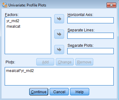
Let’s now look at the profile plots. Under Univariate click on Plots. Shift the variables mealcat to the Horizontal Axis box and yr_rnd2 into the Separate Lines box. Alternatively you can specify yr_rnd2 into the Horizontal Axis with mealcat in Separate Lines, although this would produce a different plot (try for yourself).
Click Add to shift plot down into the Plots box. Note that essentially this is plotting the interaction without actually specifying it in our model. The * symbol denotes interaction or cell means.
The code you obtain from pasting the synatx is shown below:
		UNIANOVA api00 BY yr_rnd2 mealcat
		/METHOD=SSTYPE(3)
		/INTERCEPT=INCLUDE
		/PLOT=PROFILE(mealcat*yr_rnd2)
		/PRINT=PARAMETER
		/CRITERIA=ALPHA(.05)
		/DESIGN=yr_rnd2 mealcat.
You can see that the lines are parallel to each other, which is what we expect if we do not fit an interaction model.
3.5 Regresesion with the interaction of two categorical predictors
Suppose that we think the Year Round effect changes by levels of socioeconomic status. My hypothesis is that lower SES schools will have a larger Year Round effect. To test whether this is true, we will fit a regression model where we see if the interaction of Meal Category and Year Round is a significant predictor of academic performance. Let’s use the exact same model we fit for the main effects model, entering in yr_rnd2 and mealcat as Nominal variables in the Fixed Factor(s) box. Except that now, since we want the interaction of these two predictors, click on Model and under Specify Model click on Full Factorial. This specifies the two effects of yr_rnd2 and mealcat as well as the interaction term yr_rnd2*mealcat. The beauty of using the General Linear Model in SPSS is that we don’t need to manually create our own interaction terms.
The syntax is shown below:
	UNIANOVA api00 BY yr_rnd2 mealcat
	/METHOD=SSTYPE(3)
	/INTERCEPT=INCLUDE
	/PRINT=PARAMETER
	/CRITERIA=ALPHA(.05)
	/DESIGN=yr_rnd2 mealcat yr_rnd2*mealcat.
The output we obtain from the syntax is shown below:
| Value Label | N | ||
| Year Round Recoded | 1 | Year Round | 92 |
| 2 | Not Year Round | 308 | |
| Percentage free meals in 3 categories | 1 | 0-46% free meals | 131 |
| 2 | 47-80% free meals | 132 | |
| 3 | 81-100% free meals | 137 | |
|
||||||
| Source | Type III Sum of Squares | df | Mean Square | F | Sig. | |
| Corrected Model | 6204727.822a | 5 | 1240945.564 | 261.609 | .000 | |
| Intercept | 56354756.653 | 1 | 56354756.653 | 11880.384 | .000 | |
| yr_rnd2 | 99617.371 | 1 | 99617.371 | 21.001 | .000 | |
| mealcat | 1796232.798 | 2 | 898116.399 | 189.336 | .000 | |
| yr_rnd2 * mealcat | 10583.519 | 2 | 5291.759 | 1.116 | .329 | |
| Error | 1868944.176 | 394 | 4743.513 | |||
| Total | 175839633.000 | 400 | ||||
| Corrected Total | 8073671.998 | 399 | ||||
| a. R Squared = .769 (Adjusted R Squared = .766) | ||||||
|
|||||||
| Parameter | B | Std. Error | t | Sig. | 95% Confidence Interval | ||
| Lower Bound | Upper Bound | ||||||
| Intercept | 521.493 | 8.414 | 61.978 | .000 | 504.950 | 538.035 | |
| [yr_rnd2=1] | -33.493 | 11.771 | -2.845 | .005 | -56.635 | -10.350 | |
| [yr_rnd2=2] | 0a | . | . | . | . | . | |
| [mealcat=1] | 288.193 | 10.443 | 27.597 | .000 | 267.662 | 308.724 | |
| [mealcat=2] | 123.781 | 10.552 | 11.731 | .000 | 103.036 | 144.526 | |
| [mealcat=3] | 0a | . | . | . | . | . | |
| [yr_rnd2=1] * [mealcat=1] | -40.764 | 29.231 | -1.395 | .164 | -98.233 | 16.704 | |
| [yr_rnd2=1] * [mealcat=2] | -18.248 | 22.256 | -.820 | .413 | -62.003 | 25.508 | |
| [yr_rnd2=1] * [mealcat=3] | 0a | . | . | . | . | . | |
| [yr_rnd2=2] * [mealcat=1] | 0a | . | . | . | . | . | |
| [yr_rnd2=2] * [mealcat=2] | 0a | . | . | . | . | . | |
| [yr_rnd2=2] * [mealcat=3] | 0a | . | . | . | . | . | |
| a. This parameter is set to zero because it is redundant. | |||||||
Let’s first take a look at the dummy coding table to make sense of the Parameter Estimates.
| Values | ||||||||||||
| Year Round | Meal Category | Year Round * Meal Category | ||||||||||
| Variable | Yes | No | First | Second | Third | Yes*First | Yes*Second | Yes*Third | No*First | No*Second | No*Third | |
| Year Round | Dummy1 | 1 | 0 | |||||||||
| Dummy2 | 0 | 1 | ||||||||||
| Meal Category | Dummy3 | 1 | 0 | 0 | ||||||||
| Dummy4 | 0 | 1 | 0 | |||||||||
| Dummy5 | 0 | 0 | 1 | |||||||||
| Year Round* Meal Category | Dummy6 | 1 | 0 | 0 | 0 | 0 | 0 | |||||
| Dummy7 | 0 | 1 | 0 | 0 | 0 | 0 | ||||||
| Dummy8 | 0 | 0 | 1 | 0 | 0 | 0 | ||||||
| Dummy9 | 0 | 0 | 0 | 1 | 0 | 0 | ||||||
| Dummy10 | 0 | 0 | 0 | 0 | 1 | 0 | ||||||
| Dummy11 | 0 | 0 | 0 | 0 | 0 | 1 | ||||||
There are two dummy variables for Year Round, three dummy variables for meal category and 2*3 = 6 dummy variables for the product terms, 2 + 3 + 6 = 11. We can see within each variable there is one reference group. Additionally, any product term that involves the reference group is omitted (highlighted in green). In other words, if a particular Dummy variable has a ‘1’ down a column with green, it is omitted from the analysis. This means that Dummy variables 2, 5, 8, 9, 10 and 11 will all be excluded and a zero will be put in its place when we see the SPSS output. The rule is basically to exclude any term or product term that includes the reference category, in this case Not Year Round and the Third Meal Category.
Interpreting Coefficients and Calculating Predicted Values
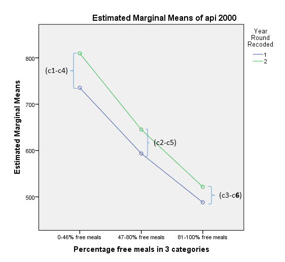
The meaning of the coefficients change in the presence of these interaction terms. For example, in the prior model, with only main effects, we could interpret [yr_rnd2=1] as Year Round effect holding mealcat constant. However, now that we have added an interaction term, the term [yr_rnd2=1] represents the difference between c3 and c6, or the effect of year-round school for mealcat = 3 (because it is the reference group). The presence of an interaction would imply that the Year Round effect depends on the levels of mealcat. The interaction terms [yr_rnd2=1]*[mealcat=1] and [yr_rnd2=1]*[mealcat=2] represent the changes in the Year Round effect going from one meal category to the third (reference) meal category. For example, the coefficient for [yr_rnd2]*[mealcat=1] represents the change in the Year Round effect when going from the lowest meal category to the highest. Another way to look at it is that [yr_rnd2]*[mealcat=1] is (c1-c4) – (c3-c6), or it represents how much the effect of yr_rnd2 differs between mealcat=1 and mealcat=3. If you compare this to the main effects model, you will see that not only are the predicted means themselves different, but that the differences between year round and non-year round schools varies by mealcat. See the profile plot at the end of this section for a visual representation of the concepts we just discussed. Adding the interaction terms in fact allows the effect of yr_rnd2 to change by levels mealcat (technically, it is also that the effect of mealcat to change by levels yr_rnd2 since the effect is symmetric but we will not go there!).
Now that we know what the coefficients mean, we can calculate the cell means. The table below shows the predicted api00 scores for the six cells in terms of the coefficients in the model.
| Meal Cat 1 | Meal Cat 2 | Meal Cat 3 | |
| Year Round | Intercept | Intercept | Intercept |
| + [yr_rnd2=1] | + [yr_rnd2=1] | + [yr_rnd2=1] | |
| + [mealcat=1] | + [mealcat=2] | ||
| +[yr_rnd2=1] * [mealcat=1] | +[yr_rnd2=1] * [mealcat=2] | ||
| 735.429 | 593.533 | 488 | |
| c1 | c2 | c3 | |
| Non Year Round | Intercept | Intercept | Intercept |
| + [mealcat=1] | + [mealcat=2] | ||
| 809.685 | 645.274 | 521.493 | |
| c4 | c5 | c6 |
Let’s recreate the difference of differences table just as we did for the main effects model.
| Year Round | ||||
| Meal Cat 1 | Meal Cat 2 | Meal Cat 3 | ||
| Non Year Round | Meal Cat 1 | -74.26 | ||
| (c1-c4) | ||||
| Meal Cat 2 | -51.74 | |||
| (c1-c4)-(c2-c5) | (c2-c5) | |||
| Meal Cat 3 | -40.76 | -18.25 | -33.49 | |
| (c1-c4) – (c3-c6) | (c2-c5) – (c3-c6) | (c3-c6) | ||
The diagonal cells are the simple effect of yr_rnd2 for a particular category of mealcat. Empty boxes are cell differences that were omitted for simplicity. Remember that for the main effects model, each of the diagonals had the same value. However, in this interaction model, you can see that the value for each cell on the diagonal is different from others. This is because an interaction means that the effect of yr_rnd2 is allowed to vary across levels of mealcat (these are the diagonal elements). The term [yr_rnd2=1] in the Parameter Estimates table matches the blue cell because it is the Year Round effect for the reference group, mealcat=3. The green cells represent the difference of differences in the Parameter Estimates output. The coefficient for [yr_rnd2=1] * [mealcat=1] = -40.76 represents the difference in the Year Round effect between the first and third meal category. The coefficient for [yr_rnd2=1] * [mealcat=2] = -18.25 represents the difference in the Year Round effect between the second and third category. Magically, you can see that adding the value of the blue cell to each of the green cells adds up to the diagonal cells! For example, -33.49 – 18.25 = -51.74 and -33.49 – 40.76 = -74.25.
Let’s take a look at the profile plots to visualize these differences of differences. The green line represents Non Year Round schools and the blue line represents Year Round schools. For each of the meal categories, the vertical differences represent the change in predicted api00 scores between year-round and non year-round schools.
Looking at the profile plots we confirm that the lines are no longer completely parallel, although since the interaction is not significant, there isn’t a huge difference from the previous profile plot where we only included the main effects. Although this section has focused on how to handle analyses involving interactions, these particular results show no indication of interaction. We could decide to omit interaction terms from future analyses having found the interactions to be non-significant. This would simplify future analyses, however including the interaction term can be useful to assure readers that the interaction term is non-significant.
(Optional)Getting the cell means
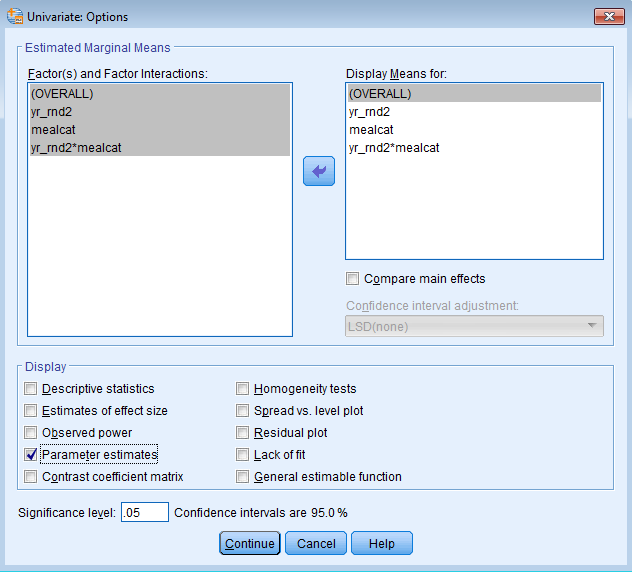
Instead of calculating the predicted api00 scores ourselves, and supposing we want the estimated means for categories besides the reference category, we should request the EMMEANS (or estimated marginal means). Go to Options and shift the (OVERALL), yr_rnd2, mealcat and yr_rnd2*mealcat terms from the Factors & Covariates left-hand box to the Model right-hand box. Make sure under the Display section that the box next to Parameter estimates are checked so we can obtain the regression coefficients. Unfortunately, the General Linear Model commands in SPSS do not give you Standardized Beta coefficients. If you need them, you will have to manually standardize the coefficients and re-run the model with the new standardized variables.
To recreate the profile plot above, under Univariate click on Plots. Shift the variables mealcat to the Horizontal Axis and yr_rnd2 into the Separate Lines box. The code you obtain is shown below:
	UNIANOVA api00 BY yr_rnd2 mealcat
	/METHOD=SSTYPE(3)
	/INTERCEPT=INCLUDE
	/PLOT=PROFILE(mealcat*yr_rnd2)
	/EMMEANS=TABLES(OVERALL)
	/EMMEANS=TABLES(yr_rnd2)
	/EMMEANS=TABLES(mealcat)
	/EMMEANS=TABLES(yr_rnd2*mealcat)
	/PRINT=PARAMETER
	/CRITERIA=ALPHA(.05)
	/DESIGN=yr_rnd2 mealcat yr_rnd2*mealcat.
The additional output you obtain from code above is shown below:
Estimated Marginal Means
|
||||
| Mean | Std. Error | 95% Confidence Interval | ||
| Lower Bound | Upper Bound | |||
| 632.236 | 5.800 | 620.832 | 643.639 | |
|
|||||
| Year Round Recoded | Mean | Std. Error | 95% Confidence Interval | ||
| Lower Bound | Upper Bound | ||||
| 1 | 605.654 | 10.861 | 584.301 | 627.007 | |
| 2 | 658.817 | 4.077 | 650.802 | 666.833 | |
|
|||||
| Percentage free meals in 3 categories | Mean | Std. Error | 95% Confidence Interval | ||
| Lower Bound | Upper Bound | ||||
| 0-46% free meals | 772.557 | 13.378 | 746.256 | 798.859 | |
| 47-80% free meals | 619.403 | 9.444 | 600.836 | 637.971 | |
| 81-100% free meals | 504.746 | 5.886 | 493.175 | 516.317 | |
|
||||||
| Year Round Recoded | Percentage free meals in 3 categories | Mean | Std. Error | 95% Confidence Interval | ||
| Lower Bound | Upper Bound | |||||
| 1 | 0-46% free meals | 735.429 | 26.032 | 684.250 | 786.607 | |
| 47-80% free meals | 593.533 | 17.783 | 558.572 | 628.495 | ||
| 81-100% free meals | 488.000 | 8.232 | 471.816 | 504.184 | ||
| 2 | 0-46% free meals | 809.685 | 6.185 | 797.526 | 821.845 | |
| 47-80% free meals | 645.274 | 6.367 | 632.755 | 657.792 | ||
| 81-100% free meals | 521.493 | 8.414 | 504.950 | 5538.035 | ||
(Optional)Calculating Marginal Means
Just as for the main effects model we can get the marginal means (Tables 2 and 3), by averaging of the cell means across the rows or down the columns. The grand mean is the average of all six cells means.
| Meal Cat 1 | Meal Cat 2 | Meal Cat 3 | |||
| Year Round | 735.429 | 593.533 | 488 | 605.654 | Averaged across mealcat |
| Non Year Round | 809.685 | 645.274 | 521.493 | 658.817 | |
| 772.557 | 619.404 | 504.747 | 632.236 | Grand Mean | |
| Averaged across yr_rnd2 | |||||
3.6 Summary
This lesson covered techniques for running regression with Nominal (i.e., categorical) predictors. We began with an introduction to dummy coding. Then, we explored the equivalency of a regression with two categories to the independent t-test and Univariate ANOVA with two groups. This allowed us to understand that we can fit linear regression models with categorical variables under a General Linear Model framework. We then proceed with our analysis of two and three category variables using the General Linear Model (i.e., the UNIANOVA command in SPSS) and we then build our model progressively by including their main effects, and then an interaction between the two variables.
The REGRESSION command can be used if you manually code the dummy variables and product (interaction) terms. The UNIANOVA (Univariate ANOVA) command will automatically create dummy variables and interaction terms for you. Using the General Linear Model allows for the simple creation of product (interaction) terms and for the easy calculation of estimated marginal or cell means. In general, a General Linear Model is preferred over a Linear Regression when categorical (Nominal) predictors are involved, but it requires a nuanced understanding of how SPSS internally creates dummy variables. Of special note is that SPSS automatically sets the highest category of a Nominal variable to the reference group, and careful interpretation of the coefficients is necessary to make correct conclusions.


