NOTE: This seminar was created using SPSS version 16.0.2. Some of the syntax shown below may not work in earlier versions of SPSS.
Here are links for downloading the data files and the syntax file associated with this seminar.
- The data set called https://stats.idre.ucla.edu/wp-content/uploads/2016/02/data08.sav .
- The data set called https://stats.idre.ucla.edu/wp-content/uploads/2016/02/data08.xls .
- The data set called /spss/seminars/spss_syntax08/data08.dta .
- The data set called https://stats.idre.ucla.edu/wp-content/uploads/2016/02/data08.sas7bdat .
- The SPSS program shown in this seminar.
Here are links for the online movies presenting the material in this seminar (under construction!!).
- Online movie for the seminar, part 1
- Online movie for the seminar, part 2
- Online movie for the seminar, part 3
- Online movie for the seminar, part 4
- See how we made these movies
Introduction
The purpose of this seminar is to help you learn about the use of SPSS syntax as an alternative to the point-and-click interface. In many instances, you may find that using syntax is simpler and more convenient than using point-and-click. The use of syntax is very useful when doing data management. One reason is because you can do repetitive tasks much quicker than you can using the point-and-click interface. You can also see what you have typed, so you don’t have to point-and-click your way back to some window to be sure that you typed the correct variable label, for example. The use of syntax is also helpful in documenting your analysis. It is difficult to take adequate notes on modifications made to the data and the procedures used to do the analyses when using the point-and-click interface. However, documenting what you are doing in a syntax file is simple, and this makes reviewing and/or reconstructing the analysis much easier.
All SPSS procedures and commands are executed using syntax, whether you use the point-and-click interface or write your own syntax. Almost everything that you can do in SPSS via point-and-click can be accomplished by writing syntax. (There are a few exceptions, most notably when using the graph editors.) Also, there are a handful of commands that are available via syntax that are not available via the point-and-click interface, such as temporary and manova. There are several ways in which you can get SPSS to show you the syntax that it is using to run your analyses, and they are explained below.
Perhaps the simplest way to ease yourself into writing SPSS syntax is to notice the syntax that SPSS includes above the results in your output file. In other words, SPSS prints the syntax of each procedure immediately above the results. If you are doing data management that does not produce results (such as creating a new variable or sorting your data), then you simply see the syntax in the output window. You can copy and paste that syntax from the output window into your syntax file so that you have a complete record of your analysis. If you would rather have the syntax go directly to the syntax file, you can click on the Paste button instead of the OK button after you have set up your analysis. This will paste the syntax that SPSS uses to run your analysis into a syntax window from which you can run the commands.
Commands in the output file
If for some reason the commands are not shown in your output file, it is
easy to have this done.
To make this change, from the Data Editor window, click on Edit, then on
Options, and then on the View tab. In the lower left-hand corner, check
the option that says "Display commands in log", and you will see all of the commands issued from then on in
your output window immediately above the corresponding output.
The SPSS journal
Finally, you can change the general SPSS options to save the SPSS
journal to a convenient location. The journal is a log of all of the SPSS
commands that have been issued, but with no output. To make this change in
SPSS versions 15 and earlier,
from the Data Editor window, click on Edit, then Options, and under the General
tab, you will see where SPSS is saving the journal file. In SPSS version
16, from the Data Editor window, click on Edit, then Options, and under the File
Locations tab, you will see where SPSS is saving the journal file. You can change
that location, and you can indicate whether the journal should be overwritten
every time you start SPSS, or if your next session should be appended to the
bottom of the existing file. You can view the journal file using a text editor such
as WordPad. Be aware that the file might be quite long, so NotePad may
not be able to open the file.
How to open a new or existing syntax file
To open a new syntax file, from the Data Editor window, click on "File", then "New", and then
"Syntax." If you want to open an existing syntax file, you would click on
"File", then "Open", and then on "Syntax". A
syntax file is nothing more than a text file; hence, you can type commands and
comments into it, and you can cut-and-paste in it as you would in any text
editor. Unlike other types of SPSS files (such as data files), you can
open syntax files in any text editor, such as WordPad or NotePad.
How to run (execute) syntax
Now that you have commands in your syntax file, how you run them?
You have several options. You can highlight one or more commands and click on
Run at the top of the syntax window. You can then select All,
Selection, Current, or To End. You can highlight one or more commands
(including the period at the end) and click on the right-pointing arrow at the
top of the syntax editor. If you want to run only one command, you can
simply put your curser anywhere in the command and click on the right-pointing
arrow. SPSS while highlight and run that command. If you would
rather not mouse to the top of the syntax window, you can press Alt-R on your
keyboard (after highlighting the command or commands that you wish to run).
Multiple open data sets
As of version 14, SPSS allows you to have multiple data sets open at once.
The syntax that you run will be run on the "active" data set. The "active"
data set is the one that is last one that you clicked on. If you get
strange error messages when you run your syntax, you may have run the syntax on
the wrong data file. If you did and you made changes to the data set that
you did not want to make, simply close the data set without saving it.
This brings up a good point: you should always work on a copy of your
data, not on the original. Keep the original somewhere safe where it
cannot be overwritten. If you make a mistake on the copy, it is no big
deal; you just make another copy of the original and continue working on that.
SPSS has a command that allows you to control which data set is active via syntax (cleverly called dataset activate). We will explore the dateset commands in the second part of this seminar. To keep things simple, we are going to have only one data open at a time in this seminar.
A comment on comments
One of the most important things to remember when writing SPSS syntax is
that all commands must end in a period (.). This includes comments, which
you can use pretty much anywhere in your syntax file. To start a comment,
use either an asterisk (*) or the command comment. If you forget to
end your comment with a period, SPSS will consider everything between comment
or * and the next period to be part of the comment, and you may be left
wondering why some of your commands did not run.
1. Opening data files
Perhaps the first thing that you need to know when using SPSS syntax is how to open a data file. The SPSS command for this is get file followed by the path where the file is located. The path and file name must be enclosed in quotes, and you need to include the file extension, which is .sav for SPSS data files.
get file "d:data08.sav".
If your data file is not in SPSS format, you may still be able to open it in SPSS. If you have an Excel file, you can type
get data
 /type = xls
 /file = 'd:data08.xls'.
Please note that there can be some issues when opening in Excel file in SPSS. One common issue is that Excel will allow you to do things that SPSS (or any other statistical package) will not. For example, you can put graphs and figures in the middle of your Excel spreadsheet, but such spreadsheets cannot be opened in SPSS. Excel allows you to use spaces in variable names, and this is not permitted in SPSS.
If your data file is in Stata format, you can type
get stata file = 'd:data08.dta'.
Please note that according to the SPSS 16 documentation, only version 4-8 Stata data files can be read into SPSS. However, I have found that I can open most Stata 9 files with SPSS 16, but not Stata 10 files.
If your data file is in SAS format, you can type
get sas data = 'd:data08.sas7bdat'.
Please note that when using the get stata command, you need to use the file keyword. When using the get sas command, you need to use the data keyword.
SPSS can also open other kinds of files, such as .csv files. These are text files that have a comma or tab delimiter (in other words, the values of the variables are separated by either a comma or a tab).
A note about quotes
You can use either single or double quotes, as
shown above, as long as they match (obviously). Quotes must be used
if you have spaces anywhere in your path specification or data file name.
For example, "D:my dissertationmy datathe current data set.sav". If you
omit the quotes, you will get an error message, and SPSS won’t open your data
file.
2. Saving an SPSS data file
You can save your SPSS data files with the save outfile command. All you need after the command is the path and the name of the new data set.
There are several handy subcommands that you can use when saving your data file. For example, you can use the keep subcommand. As you would expect, you list the variables that you want to save in the new data set on the keep subcommand. You can order them in any order that you want them in the new data set. In this example, we move the variables age and yrs_edu so that they are the first variables in the new data set (called mydata.sav), and then we keep all of the other variables in the order in which they appear in the old data set (data.sav) by using the SPSS keyword all. We will discuss the use of keywords a little later on in the seminar. If you want to eliminate a few variables from the new data set, you can use the drop subcommand and list the variables that should not be included in the new data set.
* save the data file just as it is, but with a new name.
save outfile "D:mydata.sav".
* save the data file with a new name and reorder the variables.
save outfile "D:mydata.sav"
 /keep = age yrs_edu gender all.
* save the data file with a new name and drop some variables.
save outfile "D:mydata.sav"
 /drop = str1 str2 str3.
3. Creating numeric variables
Now that we have our data file (https://stats.idre.ucla.edu/wp-content/uploads/2016/02/data08.sav) read into SPSS, let’s create some new variables. Two commands that you can use to create numeric variables are compute and if. Be aware that there is no "then" in SPSS syntax. SPSS will not create the new variables unless we issue either the execute command or a procedural command. Examples of procedural commands are list, regression and crosstabs. The procedure does not have to use the newly created variable. In many of the examples below, the execute command is technically unnecessary because we issue the procedural command list immediately afterward. However, including the execute does not cause any problems, and it is handy to have in case you later change the program and remove the command that executes the compute commands.
In the first example, we show how to make a new variable that is a copy of a variable already in the data set. We create a new variable, creatively named new_var, and set it equal to old_var. In the second example, we create a variable called newvar123 and set it equal to a constant. In our example, we set newvar123 equal to 0. At this point, every case in the data set has a value of 0. Next, we use some if commands to change the values of newvar123 according to the values in the variables num1 and num2.
The point of the following examples is that you can make the rules for value assignments as complicated as you need them to be. You can use multiple and or or conditions in a single compute or if command. Another point to be made involves the use of parentheses. How you use parentheses can affect the resulting variable. Notice that the third and fourth if command are the same, except for the use of the parentheses. The value of newvar123 is changed so that you can see the effect of the parentheses.
* compute new_variable = old_variable.
compute new_var = old_var.

compute newvar123 = 0.
if num1 = 20 newvar123 = 1.
if num1 ge 50 or num2 <= 70 newvar123 = 2.
if num1=96 and num2 = 96 or num2 = 36 newvar123 = 3.
if num1=20 and (num2 = 96 or num2 = 30) newvar123 = 4.
execute.
list num1 num2 old_var new_var newvar123.
    num1     num2  old_var  new_var newvar123

   20.00    20.00     1.00     1.00      2.00
   20.00    30.00     2.00     2.00      4.00
   52.00    36.00     3.00     3.00      3.00
   63.00    86.00     4.00     4.00      2.00
   45.00    72.00     5.00     5.00       .00
   93.00    12.00     6.00     6.00      2.00
   28.00    15.00     4.00     4.00      2.00
   75.00    46.00     5.00     5.00      2.00
   96.00    96.00     6.00     6.00      3.00
   34.00    36.00     1.00     1.00      3.00
   73.00    32.00     2.00     2.00      2.00
   20.00    30.00     3.00     3.00      4.00
   55.00    13.00     4.00     4.00      2.00
   91.00    29.00     5.00     5.00      2.00
   78.00    30.00     6.00     6.00      2.00

Number of cases read:  15    Number of cases listed:  15
You can use either symbols or letters to specify equality or inequality. Which you use is simply a matter of personal preference. Note that spacing between variables and symbols is also a matter of preference.
| Equal to | Not equal | Less than | Less than or equal to | Greater than | Greater than or equal to |
| = | ~= <> | < | <= | > | >= |
| eq | ne | lt | le | gt | ge |
You can use all sorts of math and functions when creating your variables.
compute mult_num1_num2 = num1*num2.
compute div_num1 = num1/6.56.
* click on the values of div_num1 in the data editor.
compute sum_num1_num2 = sum(num1,num2).
exe.
list mult_num1_num2 div_num1 sum_num1_num2
 /cases from 1 to 10.
mult_num1_num2 div_num1 sum_num1_num2

     400.00        3.05       40.00
     600.00        3.05       50.00
    1872.00        7.93       88.00
    5418.00        9.60      149.00
    3240.00        6.86      117.00
    1116.00       14.18      105.00
     420.00        4.27       43.00
    3450.00       11.43      121.00
    9216.00       14.63      192.00
    1224.00        5.18       70.00

Number of cases read:  10    Number of cases listed:  10
In the next example, we will create a new variable called degree, and we will set it equal to missing. Then, we will use if commands to change the missing values to the values that we want. Initially setting a new variable to missing is often a good idea when there are missing values in the original variable, so that when you are done recoding, you have missing values in your recoded variable where you had missing values in the original variable. In other words, if a case has a missing value in the original variable, you want it to have a missing value in the new variable as well. This is also a good way to see if your recoding works as you expect: if you have more missing values in your new variable than in your old variable, you will know that the recoding did not work as planned. Also notice that we can shorten execute to exe.
compute degree = $sysmis.
execute.
if yrs_edu = 12 or yrs_edu = 13 degree = 1.
if yrs_edu gt 13 and yrs_edu lt 16 degree = 2.
if yrs_edu = 16 or yrs_edu = 17 degree = 3.
if yrs_edu = 18 degree = 4.
if yrs_edu ge 19 degree = 5.
exe.
list yrs_edu degree.
 yrs_edu   degree

   13.00     1.00
   12.00     1.00
   16.00     3.00
   18.00     4.00
   12.00     1.00
   16.00     3.00
   18.00     4.00
   20.00     5.00
   15.00     2.00
   14.00     2.00
   16.00     3.00
   16.00     3.00
   18.00     4.00
   17.00     3.00
     .        .

Number of cases read:  15    Number of cases listed:  15
A note on naming variables
In the preceding examples, the naming of the variables has not been terribly
good. We do not suggest that you name your variables num1, num2,
etc. Rather, it is good practice to name your variables something
meaningful (and easy for you to type). Variable names can be up to 64 bytes long (approximately 64
characters long). However, please remember that you cannot use spaces in a
variable name, and variable names should not have an underscore at the end, as
these might conflict with variables created by commands or procedures.
Variable names should also not end with a period, as the period is the command
terminator in SPSS. (In other words, the period tells SPSS where each
command ends.) You can use any combination of upper and lower case letters
in a variable name, but SPSS is case insensitive. In other words, the
variable name might be VarName, but you can type varname, VARname or VARNAME in
the syntax, and it will work fine.
4. Creating standardized variables
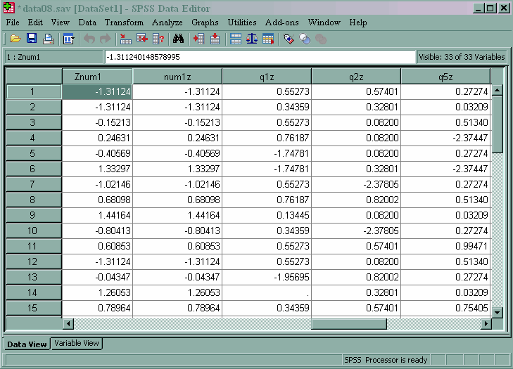
Creating standardized variables in SPSS is very simple. You can use the descriptives command with the save subcommand. If you want to name the new standardized variable instead of using the SPSS default name, you can put that name in parentheses after the variable you wish to standardize. You can also create multiple standardized variables in a single call to descriptives.
descriptives num1
 /save.
desc num1 (num1z)
 /save.
desc q1 (q1z) q2 (q2z) q5 (q5z)
 /save.
Note that a variable label was automatically created for the new variables. We also see that the command descriptives is another command that can be shortened (to desc).
5. Creating string variables
Up through version 15 of SPSS, there are two types of string variables in SPSS: short strings and long strings. Short string variables have a maximum length of eight characters. Long string variables have a maximum length of 255 characters. Long strings can be displayed by some procedures and the print command, and they can be used as "break" variables. However, long string variables cannot be used in tabulation procedures, and they cannot have user-defined missing values (see below). This means that long string variables cannot have missing values, as user-defined missing is the only kind of missing values a string variable can have.
To create either type of string variable, you usually need to use the string command. You can then populate the new string variable using the compute command. This is unlike numeric variables, which can be both created and populated using the compute command.
When creating either type of string variable (short or long), you need to indicate how long the string variable should be. This is done by including the desired length in parentheses after the name of the new string variable. You also need to include the letter "A" before the length to indicate that you want to create an alphanumeric variable (as opposed to a hexadecimal variable, which would use AHEX).
As of version 16, the distinction between short and long strings has been eliminated, the maximum length of a string variable has been increased to 32,767 characters, and string variables of all lengths can have user-defined missing values. Starting with version 16, if you wish to alter the length of a string variable, you can use the alter type command. We will see an example of this command a little later in the seminar.
string string1 (A4).
string string2 to string4 (A5).
compute string1 = "a".
if newvar123 <= 2 string1 = "B".
if str1 = "c" or str1 = "f" string1 = "c".
exe.
list newvar123 str1 string1.
newvar123 str1     string1

     2.00 a        B
     4.00 b        a
     3.00 c        c
     2.00 a        B
      .00 f        c
     2.00 d        B
     2.00 c        c
     2.00 a        B
     3.00 a        a
     3.00 c        c
     2.00 b        B
     4.00 b        a
     2.00 b        B
     2.00 f        c
     2.00          B

Number of cases read:  15    Number of cases listed:  15
6. The keyword "to"
When creating variables, the SPSS keyword to will create variables with consecutive numbering. When using to in syntax to refer to variables that already exist in the data set, SPSS assumes that variables are positionally consecutive (all variables between the first variable listed and the last variable listed in the command will be included). There are some commands in SPSS that will use the keyword to in both a positionally and a numerically consecutive manner, depending on whether existing variables are being modified in some way or whether new variables are being created. Some of these commands include autorecode, recode, aggregate and rename variables.
autorecode v1 to v2 /into w1 to w3.
rename variables (string1 to string4 = s1 to s4).
compute z = mean(q1 to q5).
exe.
list v1 to v2 w1 to w3 q1 to q5 z.
      v1    puppy       v2 w1 w2 w3       q1       q2       q3       q4       q5        z

    7.00     5.00     2.00  7  4  2     3.00     3.00      .        .       2.00     2.67
    8.00     9.00     3.00  8  8  3     2.00     2.00    -9.00      .       1.00    -1.00
    5.00     6.00     6.00  5  5  6     3.00     1.00     2.00      .       3.00     2.25
    3.00     3.00     9.00  3  3  9     4.00     1.00     2.00      .      -9.00     -.50
    2.00     1.00     8.00  2  1  8    -8.00     1.00     3.00      .       2.00     -.50
    6.00     2.00     8.00  6  2  8    -8.00     2.00     1.00      .      -9.00    -3.50
    9.00     5.00     7.00  9  4  7     3.00    -9.00     4.00      .       2.00      .00
    4.00     7.00     5.00  4  6  5     4.00     4.00     2.00      .       3.00     3.25
    1.00     8.00     4.00  1  7  4     1.00     1.00     1.00      .       1.00     1.00
    8.00     7.00     2.00  8  6  2     2.00    -9.00     3.00      .       2.00     -.50
    5.00     3.00     1.00  5  3  1     3.00     3.00     2.00      .       5.00     3.25
    7.00     9.00     3.00  7  8  3     3.00     1.00     1.00      .       3.00     2.00
    4.00     6.00     6.00  4  5  6    -9.00     4.00     4.00      .       2.00      .25
    1.00     5.00     8.00  1  4  8      .       2.00     4.00      .       1.00     2.33
    2.00     1.00     7.00  2  1  7     2.00     3.00     1.00      .       4.00     2.50

Number of cases read:  15    Number of cases listed:  15
7. Recoding variables (numeric and string)
There are several ways that you can recode variables in SPSS. For example, you can use the if command, the recode command or the autorecode command. Remember that when using the if command, there is no "then" in SPSS syntax. You can create complex rules regarding how variables get recoded. You have lots of functions from which to choose, and you can do all sorts of mathematical manipulations.
if num1 = 55 num1_new = 30.
if num1 le 50 and gender = "f" num1_new = 35.
if num1 > 80 or gender = "m" num1_new = 36.
list num1 gender num1_new.
    num1 gender   num1_new

   20.00 f           35.00
   20.00 f           35.00
   52.00 f             .
   63.00 m           36.00
   45.00 m           36.00
   93.00 f           36.00
   28.00 m           36.00
   75.00 f             .
   96.00 m           36.00
   34.00 f           35.00
   73.00 f             .
   20.00 f           35.00
   55.00             30.00
   91.00 m           36.00
   78.00 m           36.00

Number of cases read:  15    Number of cases listed:  15
There are several SPSS keywords that you can use with the recode command, including lowest, lo, hi, highest, thru, sysmis, missing, else and copy. We recommend strongly that you recode your variables into new variables, just in case the recoding does not go as you planned. You can use the into option with the recode command to create the new variable into which you will recode the old variable.
recode num1 (lowest thru 60 = 1) (85 thru highest = sysmis)(else = 2) into num1_newer.
list num1 num1_new num1_newer.
    num1 num1_new num1_newer

   20.00    35.00      1.00
   20.00    35.00      1.00
   52.00      .        1.00
   63.00    36.00      2.00
   45.00    36.00      1.00
   93.00    36.00       .
   28.00    36.00      1.00
   75.00      .        2.00
   96.00    36.00       .
   34.00    35.00      1.00
   73.00      .        2.00
   20.00    35.00      1.00
   55.00    30.00      1.00
   91.00    36.00       .
   78.00    36.00      2.00

Number of cases read:  15    Number of cases listed:  15
SPSS is case-sensitive when recoding string variables. Hence, if you use upper-case letters in your recode command and have lower-case letters in your variable, nothing will happen. This includes NOT getting an error message in the output window telling you that no recoding was done.
string str1a str2a (A5).
recode s1 ("a" = "D") ("b" = "B") ("c" = ' ')(else='x') into str1a.
recode str2 ("b" = "Z") ("a" = ' ')(else = copy)  into str2a.
exe.
list s1 str1a str2a.
string str1a str2a (A5).
recode s1 ("a" = "D") ("b" = "B") ("c" = ' ')(else='x') into str1a.
recode str2 ("b" = "Z") ("a" = ' ')(else = copy)  into str2a.

>Warning # 4684 in column 56.  Text: str2a
>On the RECODE command, the list of variables following the keyword INTO
>includes a string variable which is not of sufficient width to accept the
>longest string value generated by the value specifications.  Long values will
>be truncated to the length of the variables.
exe.
list s1 str1a str2a.
s1   str1a str2a

B    x     d
a    D     c
c
B    x     Z
c          d
B    x     d
c          f
B    x     Z
a    D
c          x
B    x     x
a    D
B    x
c
B    x     Z

Number of cases read:  15    Number of cases listed:  15
Let’s talk about what this error message means. The variable str2 was a variable that was in the original data set, and it has a length of 8. The variable that we created and tried to recode str2 into, str2a, has a length of 5; hence the error message. In this case, the recoding went OK, only because the values in str2 were only one character long. Because of this, SPSS right-padded them with blank spaces. When the recode happened, SPSS deleted the last three of those blank spaces and fit str2 into the smaller size of str2a. In many cases, it will be important information instead of blank spaces that gets truncated, so let’s see how to remedy this problem. We will use the alter type command to change the length of str2a to have a length of 8.
alter type str2a (A8).
recode str2 ("b" = "Z") ("a" = ' ')(else = copy)  into str2a.
exe.
list s1 str1a str2a.
s1   str1a str2a

B    x     d
a    D     c
c
B    x     Z
c          d
B    x     d
c          f
B    x     Z
a    D
c          x
B    x     x
a    D
B    x
c
B    x     Z

Number of cases read:  15    Number of cases listed:  15
8. Changing string variables into numeric variables
The main reason to convert a string variable into a numeric variable (often called "destringing") is for use in statistical analyses, as very few analysis procedures will allow a string variable. If there are only a few values in the string variable, you can simply recode them using the recode command. You can use the convert option of the recode command only if you have numbers and/or missing values in a string variable. Another option is to use the number function with the compute command.
recode gender ("f" = 1) ("m" = 0) into sex.
recode str3 (convert) into str3_num.
compute str3_num1 = number(str3, f8.0).
exe.
list gender sex str3 str3_num str3_num1.
gender        sex str3     str3_num str3_num1

f            1.00 1            1.00      1.00
f            1.00 5            5.00      5.00
f            1.00 4            4.00      4.00
m             .00 6            6.00      6.00
m             .00 3            3.00      3.00
f            1.00 2            2.00      2.00
m             .00 9            9.00      9.00
f            1.00 8            8.00      8.00
m             .00               .         .
f            1.00 2            2.00      2.00
f            1.00 1            1.00      1.00
f            1.00 5            5.00      5.00
              .   8            8.00      8.00
m             .00 3            3.00      3.00
m             .00 5            5.00      5.00

Number of cases read:  15    Number of cases listed:  15
The autorecode command converts string variables into numeric variables. By default, the lowest value in the string variable is given a value of 1 in the new numeric variable, the next lowest value is given a value of 2, and so on. A null string is considered to be the lowest value; hence, all cases with a value of a null string will receive a value of 1 in the new numeric variable. SPSS also creates value labels for the new numeric variable, associating the numeric values with the string values. Compare variables str3_num1 and str3auto. Although both of these new variables are the numeric version of the same string variable, str3, there are some important differences between them, such as how the missing value in str3 is handled.
autorecode gender /into sex1.
autorecode str2 /into str2auto.
autorecode str3 /into str3auto.
exe.
list gender sex1 sex str2 str2auto str3 str3_num str3_num1 str3auto.
gender   sex1      sex str2     str2auto str3     str3_num str3_num1 str3auto

f          2      1.00 d            5    1            1.00      1.00     2
f          2      1.00 c            4    5            5.00      5.00     6
f          2      1.00 a            2    4            4.00      4.00     5
m          3      2.00 b            3    6            6.00      6.00     7
m          3      2.00 d            5    3            3.00      3.00     4
f          2      1.00 d            5    2            2.00      2.00     3
m          3      2.00 f            6    9            9.00      9.00     9
f          2      1.00 b            3    8            8.00      8.00     8
m          3      2.00 a            2                  .         .       1
f          2      1.00 x            7    2            2.00      2.00     3
f          2      1.00 x            7    1            1.00      1.00     2
f          2      1.00              1    5            5.00      5.00     6
           1       .                1    8            8.00      8.00     8
m          3      2.00 a            2    3            3.00      3.00     4
m          3      2.00 b            3    5            5.00      5.00     6

Number of cases read:  15    Number of cases listed:  15
If you are using SPSS version 13 or higher, there are some additional subcommands that you can use with the autorecode command. For example, the blank subcommand indicate how missing values should be handled. In our example, we use blank = missing, so the missing values will be given the highest value in the recoded variable. The group subcommand indicates that all variables listed should use the same coding scheme, which ensures that the new variables will have a consistent coding scheme.
* the two commands below work for SPSS versions 13 and higher.
autorecode str2 str3 /into str2auto2 str3auto2 /group.
autorecode str2 str3 /into str2auto3 str3auto3 /blank = missing.
exe.
list str2 str2auto str2auto2 str2auto3 str3 str3auto str3auto2 str3auto3.
display dictionary.
str2     str2auto str2auto2 str2auto3 str3     str3auto str3auto2 str3auto3

d            5        13        4     1            2         2        1
c            4        12        3     5            6         6        5
a            2        10        1     4            5         5        4
b            3        11        2     6            7         7        6
d            5        13        4     3            4         4        3
d            5        13        4     2            3         3        2
f            6        14        5     9            9         9        8
b            3        11        2     8            8         8        7
a            2        10        1                  1         1        9
x            7        15        6     2            3         3        2
x            7        15        6     1            2         2        1
             1         1        7     5            6         6        5
             1         1        7     8            8         8        7
a            2        10        1     3            4         4        3
b            3        11        2     5            6         6        5

Number of cases read:  15    Number of cases listed:  15
9. Changing numeric variables to string variables
Converting from numeric to string is a relatively uncommon task. One instance in which you may want to do this is when you want to combine values in different numeric variables to create a unique identifier. For example, let’s say that we have three numeric variables, tid1, tid2 and tid3, and these variables tell us something about the various conditions each subject was in. You could give a single value to each combination and label that value, but you might want to simply combine (concatenate) the numbers. To do this, we start by creating a string version of each variable. Next, we use the compute command with the concat function to put the values from the three variables into a single variable.
Below is the syntax for accomplishing this task. First, we create three string variables. In this example, we will give each string variable a length of 3. Next, we use the string function to convert the numeric variable into a string variable. When using the string function, we need to list the name of the numeric variable and its numeric format. You can specify almost any numeric format that you want, but you need to consider the length of the string variable into which it will go. For example, if we used the f8.2 format, only the first digit will be put into the string variable. For stid3, we could have used the format f1.0, but f2.0 was used to show the use of the ltrim function below.
If the format for the numeric variable you specify exceeds the width of the string variable, you will get an error message and no values will be added to your string variable. In such a situation, you could use either the alter type command to make the string variable wider, or the formats command to change the format of the numeric variable.
string stid1 stid2 stid3 (A3).
compute stid1 = string(tid1, f3.0).
compute stid2 = string(tid2, f3.0).
compute stid3 = string(tid3, f2.0).
exe.

string stid123 (A8).
* compute stid123 = concat(ltrim(rtrim(stid1)), rtrim(ltrim(stid2)), (ltrim(stid3))).
compute stid123 = concat(rtrim(stid1), rtrim(stid2), (ltrim(stid3))).
exe.
list stid1 stid2 stid3 stid123.
stid1 stid2 stid3 stid123

123   987    1    1239871
456   789    1    4567891
321   987    2    3219872
654   789    2    6547892
123   987    3    1239873
321   789    3    3217893
654   987    4    6549874
123   789    5    1237895
456   987    6    4569876
123   789    6    1237896
321   987    5    3219875
654   789    1    6547891
654   987    2    6549872
321   789    3    3217893
456   987    6    4569876

Number of cases read:  15    Number of cases listed:  15
10. Sorting variables
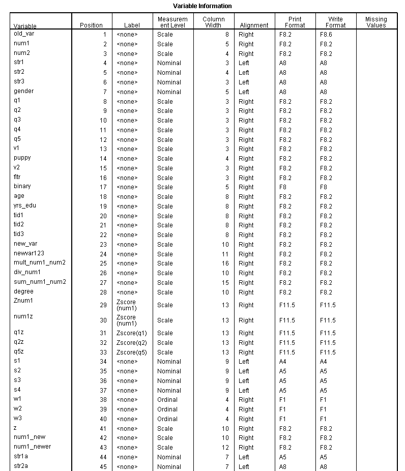
The sort variables command is new to SPSS 16. Obviously, it is a convenience command, but it is also a good way to make sure that you have done all of the data documenting that you meant to do (by sorting the variables by labels or values, for example).
sort variables by name.
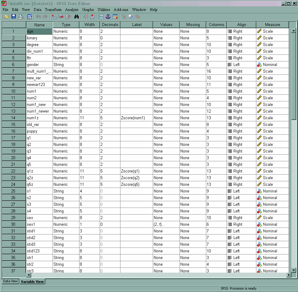
We can sort the variables in the data set in other ways, such as by type (i.e., string or numeric), or by missing.
sort variables by type.
sort variables by missing.
I am going to resort the variables by name so that it is easier to work with the data file.
sort variables by name.
11. Delete variables
The delete variables command is a very handy command, but obviously, this command needs to be used with caution. The delete variables command was introduced in version 12, so if you are using an earlier version of SPSS, you won’t be able to use this command. However, you can delete variables in any version of SPSS by highlighting them in the Data Editor and pressing the Delete key on your keyboard.
delete variables s2 s3 s4 sex1 znum1.
Another way to do the same thing is to use the save outfile command with either the keep or the drop subcommand. The difference is that with the delete variables command, you are not saving a new data file.
save outfile 'd:data08_deleted.sav'
 /drop s2 s3 s4 sex1 znum1.
12. Variable levels
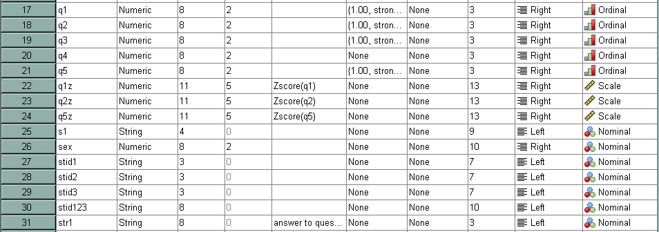
The variable levels are shown in the Variable View window of the Data Editor in the far right column. With earlier versions of SPSS, the only procedure that used the variable level was igraph, which is obviously a graphing command. However, in more recent versions of SPSS, other procedures are making use of the variable levels, so it is becoming more important that users know how to modify them. Here is a simple example.

variable level q1 to q5 (ordinal)
 /sex (nominal).

13. Documenting data
There are many ways to document your data using SPSS. There are also several commands that you can use to view the documentation that you have created, including sysfile info and display. When using the sysfile info command, you must specify the file path. Also, the maximum length of a variable label is 255 characters and the maximum length of a value label is 120 bytes (approximately 120 characters).
The document command is very handy and allows you to keep notes with your data set. In my opinion, this may be one of the most underused commands in SPSS. You can use the document drop command to remove a document from your data file.
The add document command can be used at include additional notes to your document. Unlike the document command, you will need to use quotes around each line of the text when using this command.
The file label command is another good command to remember. This is particularly useful when you have multiple copies of a data set that are slightly different.
The variable labels command allows you to assign labels to your variables. Doing so is an important part of developing a codebook. We strongly recommend that all data sets have a codebook, even if the researcher is not planning on sharing the data with others. The codebook reminds you of all of the details of your data set, which is important when you have to come back to the data at a later time.
The value labels command allows you to assign labels to the values of a variable.
You can use the add value labels command to labels values that were not labeled with the value labels command.
Using the point-and-click interface, you can check the spelling of variable labels and value labels. To do this, from the Data Editor, click on Utilities -> Spelling.
sysfile info 'd:https://stats.idre.ucla.edu/wp-content/uploads/2016/02/data08.sav'.
document I collected these data on January 16, 2003 and
blah blah blah.
add document "This is my additional comment"
"to my original document command.  Note "
"that each addition line of text must be enclosed in quotes.".
display document.
* drop documents.
file label SPSS Syntax Seminar data file.
save outfile 'd:data081.sav'.
sysfile info 'd:data081.sav'.
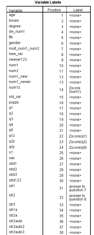
variable labels str1 'answer to question 7'
str2 'answer to question 8'.
display labels.
value labels yrs_edu 1 "high school" 2 "some college" 3 "Bachelors"
4 "Masters" 5 "Ph.D.".
value labels q1 to q3 q5 1 'strongly disagree' 2 'disagree' 3 'agree'.
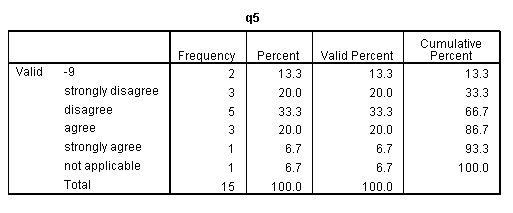
add value labels q5 4 'strongly agree' 5 'not applicable'.
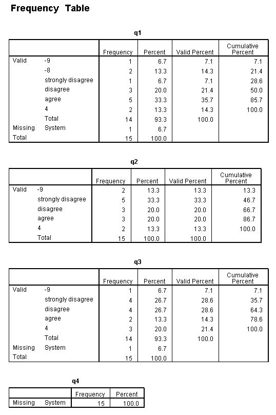
freq var = q1 to q5.
save outfile 'd:data082.sav'.
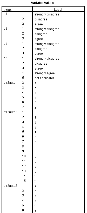
display dictionary.
14. Missing data
There are two different types of missing data in SPSS: system-missing and user-defined missing. System-missing is displayed as a dot (.) in the column of a numerical variable. String variables cannot have system-missing values; even a null string is considered a valid value. You can define your own missing values (called user-defined missing) for either numeric or (short) string variables. Missing values are considered the lowest possible value in SPSS. Although displayed differently, both system-missing and user-defined missing values are just missing values to SPSS; they are treated the same way (except in filter variables, see below). Both will be deleted from analyses that call for listwise deletion. The only "difference" is that they will be displayed in separate categories in crosstabs, frequencies, etc.
missing values q1 to q5 (-9).
missing values q3 (-7).
missing values q1 q2 (-9 -8).
missing values str1 ('x').
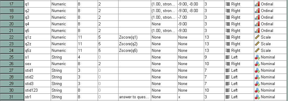
To change or remove values that have been assigned as missing you can issue the missing values command again. To remove some values and leave others, or to remove some (or all) values and reassign other values, simply issue the missing values command with the values that you want. To remove all missing values, simply leave the parentheses empty.
missing values q5 ().
It is important to realize is that you can create the same variable in different ways, and that the missing values may be handled differently. Note that above we defined -8 and -9 as missing values for the variable q1 (in the third missing values command), and -9 as a missing value for the variable q2 (in the first missing values command).
compute y = q1+q2.
compute y1 = sum(q1, q2).
exe.
list q1 q2 y y1.
      Q1       Q2        Y       Y1

    3.00     3.00     6.00     6.00
    2.00     2.00     4.00     4.00
    3.00     1.00     4.00     4.00
    4.00     1.00     5.00     5.00
   -8.00     1.00      .       1.00
   -8.00     2.00      .       2.00
    3.00    -9.00      .       3.00
    4.00     4.00     8.00     8.00
    1.00     1.00     2.00     2.00
    2.00    -9.00      .       2.00
    3.00     3.00     6.00     6.00
    3.00     1.00     4.00     4.00
   -9.00     4.00      .       4.00
     .       2.00      .       2.00
    2.00     3.00     5.00     5.00

Number of cases read:  15    Number of cases listed:  15
15. Creating and using filters (subsetting data)
Up to now, we have been focusing mostly on data management. But the reason researchers do data management is to prepare for data analysis, and very soon we will get to some data analysis. First, however, let’s talk about subsetting data, which many SPSS users call "filtering data", because in SPSS, you use the filter command to do this. So what is subsetting or filtering data?
Sometimes you want to analyze only some cases in your data set. For example, you may want to analyze only the data for males or only for females. There are several ways that you can do this in SPSS. One way is to create a variable to use as a filter variable and keep it in your data set. In constructing a variable to use as a filter variable, we suggest that you create a 0/1 (dummy) variable, where the cases with the 0s will be filtered out. It is important to note that SPSS does not treat system-missing and user-defined missing values the same way when applying the filter: cases with system-missing values will be filtered out, but cases with user-defined missing values will not. In other words, SPSS only looks for two specific values to be filtered out of your data: 0 and system-missing. You can use either the filter off command or the use all command to end the filtering of your data. A nice feature of using a filter variable is that the cases are not deleted from your data set, and if you make a mistake creating your filter variable, it is a simple matter to fix it. Remember all of those examples using the compute and if commands at the beginning of the seminar? This is a good place to use them!
filter by fltr.
desc num1 num2.

filter off.
* use all.
desc num1 num2.

The select if command will permanently delete data from your data file. The command select if is the same as using the filter in the point-and-click interface with the "delete" radio button selected.
One command that can be used only via syntax is temporary. In the syntax below, we will use the temporary command so that our observations are not permanently deleted from our data file when we use the select if command. The temporary command stays in effect only until the next executable command is executed. That is why the output for the first list command (which is the first executable command after temporary) has only seven observations (the seven that met the criteria listed on the select if command), while the second list command includes all of the observations from our data set. Although for this seminar we only use the temporary command while subsetting, it has many other uses.
temporary.
select if (gender = "f" and q1 ge 2).
list num1.
list num1.
    NUM1

   20.00
   20.00
   52.00
   75.00
   34.00
   73.00
   20.00

Number of cases read:  7    Number of cases listed:  7
    NUM1

   20.00
   20.00
   52.00
   63.00
   45.00
   93.00
   28.00
   75.00
   96.00
   34.00
   73.00
   20.00
   55.00
   91.00
   78.00

Number of cases read:  15    Number of cases listed:  15
Another command that you can use to subset your data is split file. You will first need to sort your data by the variable that will be used in the split file command. The split file command will remain in effect until you use the split file off command to turn it off.
sort cases by gender.
split file by gender.
desc num1 num2.
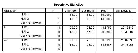
In this data set there are actually three values of gender: missing (a null string), "f" and "m". Notice also that you do not get the total for all cases.
split file off.
desc num1 num2.

16. Pasting syntax
GET
  FILE='D:https://stats.idre.ucla.edu/wp-content/uploads/2016/02/data08.sav'.

analyze - descriptives - explore.

EXAMINE
  VARIABLES=num1 BY gender
  /PLOT BOXPLOT STEMLEAF
  /COMPARE GROUP
  /STATISTICS DESCRIPTIVES
  /CINTERVAL 95
  /MISSING LISTWISE
  /NOTOTAL.

examine num1 by gender.
Notice that we get exactly the same output using both of the examine commands above. As you can see, when you paste the syntax, SPSS includes many of the default options, and these clutter the syntax. It is a good idea to play around with syntax that you have pasted to see what subcommands can be eliminated without changing the output. In the example above, all of the subcommands can be eliminated.
17. The SPSS syntax guide, AKA the SPSS Command Syntax Reference
You can access the SPSS syntax guide by clicking on "Help" and then "Command Syntax Reference" from any of the SPSS windows (the Data Editor, Syntax or Output windows).
18. The keywords "by" and "with"
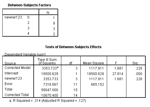
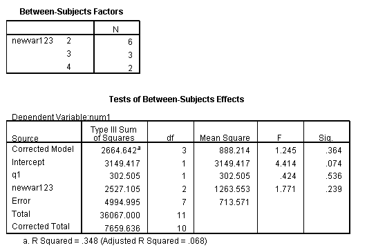
In some of the analysis commands in SPSS, the keyword by indicates that a categorical variable or variables will follow, while the keyword with indicates that a continuous variable or variables will follow. Let’s look at a few examples.
unianova num1 by newvar123.
unianova num1 by newvar123 with q1.
19. For more information
We have many Learning Modules and Frequently Asked Questions that will provide additional information:
- SPSS Learning Modules
- Creating and recoding variables
- Using SPSS functions for making/recoding variables
- Subsetting variables and observations
- How can I analyze a subset of my data?
- Labeling and documenting data
- SORT and SPLIT BY
- Missing data in SPSS
- How can I see the number of missing values and patterns of missing values in my data file?
- How do I count the number of missing values for a character variable?
- How can I get a count of how many cases are missing in a string variable?
- How can I easily convert a string variable into a categorical numeric variable?
- How do I create and modify string (character) variables?
- How can I change a string variable into a numeric variable?
- How do I standardize variables in SPSS?
We also have some books that you can check out from our Stat Books for Loan , including
- SPSS Programming and Data Management: A Guide for SPSS and SAS Users, Fourth Edition by Raynald Levesque
- An Intermediate Guide to SPSS Programming: Using Syntax for Data Management by Sarah Boslaugh
- SPSS 13.0 Guide to Data Analysis by Marija J. Norusis
- SPSS For Windows: Step by Step by Darren George and Paul Mallery
- SPSS for Psychologists, Third Edition by Nicola Brace, Richard Kemp and Rosemary Snelgar
- Next Steps with SPSS by Eric L. Einspruch
- The SPSS Book by Matthew J. Zagumny
