NOTE: This seminar was created using SPSS version 16.0.2. Some of the syntax shown below may not work in earlier versions of SPSS.
Here are links for downloading the data files and the syntax file associated with this seminar.
- The data set called https://stats.idre.ucla.edu/wp-content/uploads/2016/02/data08_2.sav.
- The data set called https://stats.idre.ucla.edu/wp-content/uploads/2016/02/kidslw-1.sav.
- The data set called https://stats.idre.ucla.edu/wp-content/uploads/2016/02/long-2.sav.
- The SPSS syntax shown in this seminar
Here are links for the online movies presenting the material in this seminar.
- Online movie for the seminar, part 1 (sections x-y) forthcoming
- Online movie for the seminar, part 2 (sections x-y) forthcoming
- Online movie for the seminar, part 3 (sections x-y) forthcoming
- Online movie for the seminar, part 4 (sections x-y) forthcoming
Introduction
In this second part of our Introduction to SPSS syntax seminar, we will see some new commands, as well as revisit some that we saw in Part 1. To get warmed up, let’s start by considering some commands that we saw in Part 1. This time, we will consider some other options, other functions, etc. We are going to illustrate these by looking at some common data management tasks. These include:
- taking a simple random sample (SRS) by creating a random number, sorting data by that random number, and taking the first few cases.
- creating a random ID variable.
- creating an index number.
- creating a flag variable for complete cases.
- creating a level-2 variable (in section 4).
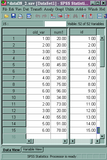
get file "d:data08_2.sav".
Before we get started on our tasks, it will be helpful to know about a type of SPSS variable called a system variable.
1. System variables
SPSS sometimes uses internal variables that you never see in the Data Editor. You can call on these internal variables, which SPSS calls "system variables," to make certain tasks easier. All system variables begin with a $. For example, SPSS keeps information about case numbers (which are the numbers that you see along the left side of the Data Editor in the gray bar) in a system variable called $casenum. You can use this variable to create an identification variable that is part of your data set.
compute id = $casenum.
exe.
list id.
Another handy system variable is $sysmis, which can be used when you want to specify that a newly created variable (or some of its values) should be set to system missing.
compute miss = $sysmis.
compute miss1 = 1.
if missing(q1) or missing(q3) miss1 = $sysmis.
exe.
list miss q1 q3 miss1.
    MISS       Q1       Q3    MISS1

     .       3.00      .        .
     .       2.00    -9.00     1.00
     .       3.00     2.00     1.00
     .       4.00     2.00     1.00
     .      -8.00     3.00     1.00
     .      -8.00     1.00     1.00
     .       3.00     4.00     1.00
     .       4.00     2.00     1.00
     .       1.00     1.00     1.00
     .       2.00     3.00     1.00
     .       3.00     2.00     1.00
     .       3.00     1.00     1.00
     .      -9.00     4.00     1.00
     .        .       4.00      .
     .       2.00     1.00     1.00

Number of cases read:  15    Number of cases listed:  15
When working with dates, a potentially useful system variable is $jdate. This variable gives the current date as the number of days from October 14, 1582. (This is a little different from dates in SPSS, which are numeric values equal to the number of seconds from midnight, October 14, 1582, which is the start of the Gregorian calendar.)
compute today = $jdate.
exe.
Task 1: Taking a simple random sample
Now let’s get back to our tasks. Our first task is to take a simple random sample. Now, we could use the sample command, but we are going to do this manually, so that we can use some functions and commands. We start by creating a random number. Next, we sort on the random number, and then we select some of the cases. As we will see, there are several ways that we can select the cases.
Before we start this task, let’s discuss why you might want to take a simple random sample of your data. One reason might be to create two or more smaller data sets that could be used for developing and then testing a model. For example, let’s say that you have a large data, perhaps 500,000 cases. You could split this file into two data (or more) sets. You would use the first data set (sometimes called the "training data set") to develop your model, and then the second data set (sometimes called the "validation" data set) to see how well the model fits that data set. Another reason you might take a simple random sample of your data is so that you can debug your syntax more quickly. If you have a large data set, it may take several minutes (or longer) for your syntax to run. If you sample your data so that you have a relatively small data set, you can test out your syntax and get any error messages quickly. Once you have a syntax file that runs without errors, you can run it on your complete data set.
Now, before we create a random number (or invoke any random process), we will "set the seed". SPSS, like almost all computer programs, uses a pseudo-random number generator. The seed is the starting point for this process. If the process of generating the random numbers starts from the same value each time, the same random numbers will be generated the syntax is run. Getting the same random numbers each time we run our syntax is important so that we can replicate our work. To set the seed in SPSS, we use the set command with the seed keyword, and then list a number. This number is the starting point for the process. It does not matter what number you select, as long as it is a positive number less than 2,000,000,000. The default (at least in SPSS version 17) is 2,000,000.
We will use the uniform function to create our random number. The argument (the number in parentheses) indicates the upper limit of the random numbers to be generated. By default, the lower limit is 0, which is why we add 1 to it. This process can generate the same number more than once, which is why we don’t use 15 as the upper limit (because it is too likely that we would get duplicate values) and don’t truncate the numbers (make them whole numbers).
set seed 156323669.
compute ran_num = uniform(100) + 1.
sort cases by ran_num.
list id ran_num.
      id  ran_num

    4.00     4.26
    6.00    29.61
   15.00    34.19
   13.00    49.33
   14.00    54.73
   12.00    55.23
    3.00    55.50
    9.00    58.89
   10.00    60.18
    5.00    75.17
    2.00    78.63
    7.00    88.11
   11.00    89.81
    1.00    98.89
    8.00   100.70

Number of cases read:  15    Number of cases listed:  15
Finally, we use three different ways to select six cases.
We will use the select if command to select the first six cases. We use the temporary command with each of them so that we don’t have to reload the data set to use the next method. If we did not use the temporary command before the select if, n of cases or sample commands, the other cases would be deleted from the data set.
temporary.
select if $casenum le 6.
list id ran_num.
      id  ran_num

    4.00     4.26
    6.00    29.61
   15.00    34.19
   13.00    49.33
   14.00    54.73
   12.00    55.23

Number of cases read:  6    Number of cases listed:  6
Here we will use the n of cases command. As with the command above, this command keeps only the first six cases in the data set.
temporary.
n of cases 6.
list id ran_num.
      id  ran_num

    4.00     4.26
    6.00    29.61
   15.00    34.19
   13.00    49.33
   14.00    54.73
   12.00    55.23

Number of cases read:  6    Number of cases listed:  6
If we use the sample command, SPSS samples 6 cases from the 15 cases in our data set. Because we set the seed previously in this session, we will select these same 6 cases if we started this process from the beginning (i.e., opened the data set and ran the syntax above).
temporary.
sample 6 from 15.
exe.
list id ran_num.
      id  ran_num

   14.00    34.19
   15.00    49.33
    5.00    58.89
    8.00    75.17
   10.00    88.11
   13.00    98.89

Number of cases read:  6    Number of cases listed:  6
Task 2: Creating a random identification variable
Our second task is to create a random identification variable. Creating a random ID variable is an important research task, because it is dangerous to have any information in a data set that could be used to identify subjects. Once you have created the random ID variable, you can create two data sets. In one data set, you keep all of the variables, and you put the data set in a safe place as a back up. In the other data set, you delete all identifying information and keep only the random ID variable. This is the data set that you use for analysis, etc.
Now, in many cases, simply assigning the case number as we did in the previous section is a sufficiently random identifier. However, if your data are sorted in some meaningful way, such as alphabetically by respondents’ last name, then you may want to sort your data in a random order before you assign the case number as the identification number. To complete this task, we will start by creating a random number, sorting the data by that random number, and then assign the case number as the random identification number. We use the case number as the random identifier and not the random number itself for two reasons. First, the case number is an integer (a.k.a., a whole number). The second reason is that there is no guarantee that the numbers produced by the pseudo-random number generator are unique. In other words, the same number may appear more than once. This problem is made worse if you truncate the decimals from the random numbers to make them whole numbers.
In this section, we are going to use a different method of creating a random variable, just to illustrate that there is more than one way to accomplish this task. We will use the rv.normal function to create the random variable. This function requires two arguments, the first being the mean of the distribution and the second being the standard deviation. You can use whatever mean and standard deviation that you like.
We will start be setting a new seed (but we technically don’t have to do this), and then creating the random variable. Next, we sort the data by this random variable, and finally, we create the identification variable using the SPSS system variable $casenum.
set seed 185693256.
compute ran_num1 = rv.normal(100, 10).
desc var = ran_num1.
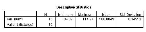
sort cases by ran_num1.
compute my_id = $casenum.
list my_id ran_num1.
   my_id ran_num1

    1.00    84.87
    2.00    89.36
    3.00    91.22
    4.00    93.16
    5.00    97.34
    6.00    98.57
    7.00   101.78
    8.00   101.84
    9.00   103.44
   10.00   104.34
   11.00   106.04
   12.00   107.99
   13.00   108.08
   14.00   109.09
   15.00   114.97

Number of cases read:  15    Number of cases listed:  15
Task 3: Creating an index number
For this task, imagine that you have a data set that has multiple observations for each subject. These data are in "long" form, meaning that each subject has multiple rows of data, one row for each observation. For example, suppose that we have data on children in families, and each family has more than one child. Hence, the data set will have a row of data for each child in the family. For data like these, you need to have two types of identification variables: one for families, and the other for children within each family. The identification variable for the children is often called an index number.
Let’s open the data set and look at it. We will create
get "d:kidslw.sav".
list famid kidname age.
    famid kidname       age

     1.00 Beth         9.00
     1.00 Bob          6.00
     1.00 Barb         3.00
     2.00 Andy         8.00
     2.00 Al           6.00
     2.00 Ann          2.00
     3.00 Pete         6.00
     3.00 Pam          4.00
     3.00 Phil         2.00

Number of cases read:  9    Number of cases listed:  9
compute index1 = 1.
if famid = lag(famid) index1 = lag(index1) + 1.
exe.
list famid index1 kidname age.
    famid   index1 kidname       age

     1.00     1.00 Beth         9.00
     1.00     2.00 Bob          6.00
     1.00     3.00 Barb         3.00
     2.00     1.00 Andy         8.00
     2.00     2.00 Al           6.00
     2.00     3.00 Ann          2.00
     3.00     1.00 Pete         6.00
     3.00     2.00 Pam          4.00
     3.00     3.00 Phil         2.00

Number of cases read:  9    Number of cases listed:  9
Task 4: Creating a flag variable for complete cases
Our last task is to create a flag variable for complete cases. A flag variable is simply is binary (0/1) variable, a.k.a. an indicator variable. You can create an indicator variable for anything in your data set; we are going to create one to indicate if a case has complete data. Knowing which cases have complete data is useful, because most procedures do a listwise deletion of incomplete cases. This means that you might be using different cases when you run analyses with different variables. If you limit all analyses to include only complete cases, you will be sure that all analyses are run on exactly the same cases.
To accomplish this task, we will start by creating a new variable called comp_flag that is equal to 1. Next, we will use the missing function to determine which cases have missing values for our variables of interest. We will also label the values of comp_flag, just to be extra clear about what the 0s and 1s mean. Please note that although we will be defining missing values for variables q1 to q5, we will only be creating the flag variable for variables q1 to q3. Setting the missing values for q4 and q5 is done here for use in a later example.
get file "d:data08_2.sav".

missing values q1 to q5 (-8 -9).
compute comp_flag = 1.
if missing(q1) or missing(q2) or missing(q3) comp_flag = 0.
value labels comp_flag 0 "has at least one missing value" 1 "complete case" .
exe.
freq var = comp_flag.
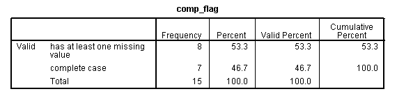
list q1 q2 q3 comp_flag.
      q1       q2       q3 comp_flag

   -8.00     2.00     1.00       .00
     .       2.00     4.00       .00
    1.00     1.00     1.00      1.00
    3.00    -9.00     4.00       .00
    2.00     3.00     1.00      1.00
    4.00     1.00     2.00      1.00
   -8.00     1.00     3.00       .00
    3.00     3.00      .         .00
    2.00     2.00    -9.00       .00
    2.00    -9.00     3.00       .00
   -9.00     4.00     4.00       .00
    4.00     4.00     2.00      1.00
    3.00     3.00     2.00      1.00
    3.00     1.00     1.00      1.00
    3.00     1.00     2.00      1.00

Number of cases read:  15    Number of cases listed:  15
Now, let’s use our indicator variable as a filter variable. We will issue the regression command and include the descriptives subcommand so that we can use the n option to see the number of cases used in the regression analysis. By doing the regression this way, we don’t use any of the cases that have a missing value for the variable q3, even though the variable q3 is not used in the regression.
filter by comp_flag.
regression
dep = q1
/method = enter q2
/descriptives = n.
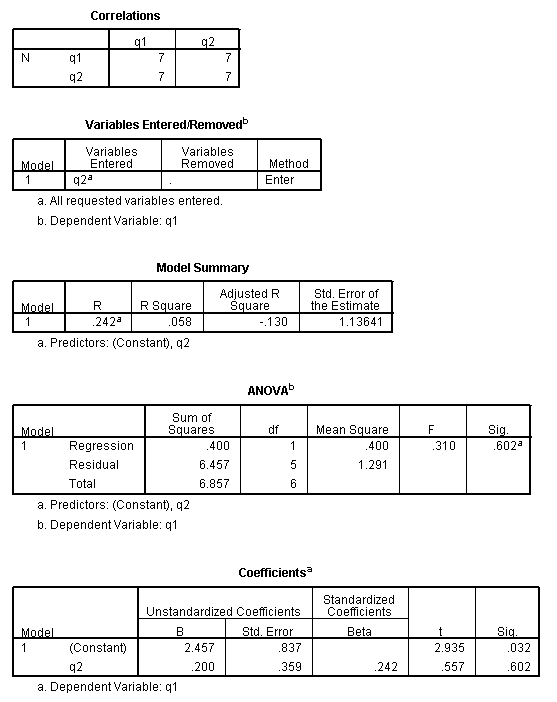
In the first table in the output above, you can see how many cases are used in the analysis. In this analysis, seven cases were used. (This can be confirmed by looking at the ANOVA table.)
When thinking about filtering out incomplete cases, you may wonder valid (i.e., non-missing) or missing values each case has for a given set of variables. This is easy to determine by using either the nvalid or nmissing functions.
use all.
* filter off.
compute nv = nvalid(q1, q2, q3).
compute nm = nmissing(q1, q2, q3).
list q1 q2 q3 comp_flag nv nm.
      q1       q2       q3 comp_flag       nv       nm

    3.00     3.00      .         .00     2.00     1.00
    2.00     2.00    -9.00       .00     2.00     1.00
    3.00     1.00     2.00      1.00     3.00      .00
    4.00     1.00     2.00      1.00     3.00      .00
   -8.00     1.00     3.00       .00     2.00     1.00
   -8.00     2.00     1.00       .00     2.00     1.00
    3.00    -9.00     4.00       .00     2.00     1.00
    4.00     4.00     2.00      1.00     3.00      .00
    1.00     1.00     1.00      1.00     3.00      .00
    2.00    -9.00     3.00       .00     2.00     1.00
    3.00     3.00     2.00      1.00     3.00      .00
    3.00     1.00     1.00      1.00     3.00      .00
   -9.00     4.00     4.00       .00     2.00     1.00
     .       2.00     4.00       .00     2.00     1.00
    2.00     3.00     1.00      1.00     3.00      .00

Number of cases read:  15    Number of cases listed:  15
As you can see in the output above, the number of valid cases (nv) and
the number of missing cases (nm) always sum to three, which they should
because there are three variables (q1, q2 and q3).
2. A little more on creating numeric variables and using numeric formats
Before we move onto other topics, let’s look at just a few examples that use the compute command. The first two examples illustrate how to work with missing values.
compute my_id = $casenum.
if sysmis(q1) and num1 < 45 or num2 > 50 newvar6 = 1.
if q3 ~= $sysmis and q1 = 1 newvar6 = 2.
exe.
The next three examples illustrate the creation of dummy (AKA binary) variables. In the first example, we create the variable dummy_var1 that is equal to 1 when the variable old_var is equal to 1 and is 0 otherwise. In the second example, we do the same thing when old_var equals 2. In the third example, we create the variable filter1, which will equal 1 when the variable my_id is equal to one of the values listed. The any function is a very handy function because it can save you lots of typing, as you can see in the syntax that is commented out.
compute dummy_var1 eq (old_var=1).
* compute dummy_var = 0.
* if old_var = 1 dummy_var = 1.
* if missing(old_var) dummy_var = $sysmis.
compute dummy_var2 = (old_var=2).
compute filter1 = any(my_id, 1, 5, 7, 9).
* compute filter2 = 0.
* if my_id = 1 or my_id = 5 or my_id = 7 or my_id = 9 filter2 = 1.
exe.
list my_id q1 num1 num2 newvar6 dummy_var1 dummy_var2 filter1.

   my_id       q1     num1     num2  newvar6 dummy_var1 dummy_var2  filter1

    1.00     3.00    20.00    20.00      .        1.00        .00      1.00
    2.00     2.00    20.00    30.00      .         .00       1.00       .00
    3.00     3.00    52.00    36.00      .         .00        .00       .00
    4.00     4.00    63.00    86.00     1.00       .00        .00       .00
    5.00    -8.00    45.00    72.00     1.00       .00        .00      1.00
    6.00    -8.00    93.00    12.00      .         .00        .00       .00
    7.00     3.00    28.00    15.00      .         .00        .00      1.00
    8.00     4.00    75.00    46.00      .         .00        .00       .00
    9.00     1.00    96.00    96.00     1.00       .00        .00      1.00
   10.00     2.00    34.00    36.00      .        1.00        .00       .00
   11.00     3.00    73.00    32.00      .         .00       1.00       .00
   12.00     3.00    20.00    30.00      .         .00        .00       .00
   13.00    -9.00    55.00    13.00      .         .00        .00       .00
   14.00      .      91.00    29.00      .         .00        .00       .00
   15.00     2.00    78.00    30.00      .         .00        .00       .00

Number of cases read:  15    Number of cases listed:  15
Of course, you can use more than one function at a time. In this example, we take the mean of five variables and round it to a whole number.
compute rnd_mean = rnd(mean(q1 to q5)).
exe.
To be complete, we should mention the numeric command. It is another way to create a new numeric variable. When using the numeric command, you can specify the format. The numeric command is like the string command in that it creates an empty variable that you then populate using the compute or if command. In the first example below, we create two new numeric variables called n1 and n2. Because we did not list a format on the numeric command, these variables have the default format, which is f5.2. This means that the variable has a length of 8, with 2 spaces after the decimal, 1 space for the decimal, and 5 spaces for integer portion of the number.
numeric n1 n2.
numeric n3 (f4.0) n4 (f8.4).
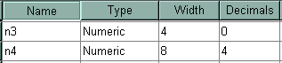
compute n3 = q1.
compute n4 = q2.
exe.
list q1 n3 q2 n4.
      q1   n3       q2       n4

   -8.00    .     2.00   2.0000
     .      .     2.00   2.0000
    1.00    1     1.00   1.0000
    3.00    3    -9.00    .
    2.00    2     3.00   3.0000
    4.00    4     1.00   1.0000
   -8.00    .     1.00   1.0000
    3.00    3     3.00   3.0000
    2.00    2     2.00   2.0000
    2.00    2    -9.00    .
   -9.00    .     4.00   4.0000
    4.00    4     4.00   4.0000
    3.00    3     3.00   3.0000
    3.00    3     1.00   1.0000
    3.00    3     1.00   1.0000

Number of cases read:  15    Number of cases listed:  15
This brings up the changing of numeric formats, which can be done with the formats command.
formats num1 (dollar6) num2 (f3.1).
list num1 num2.
  num1 num2

   $93   12
   $91   29
   $96   96
   $28   15
   $78   30
   $63   86
   $45   72
   $20   20
   $20   30
   $34   36
   $55   13
   $75   46
   $73   32
   $20   30
   $52   36

Number of cases read:  15    Number of cases listed:  15
The formats command only works with numeric variables and has no effect on your output, only the way your data look in the Data Editor.
3. String functions
We covered the creation of string variables in the Part 1 of the seminar. If necessary you can review Section 5 to refresh your memory on the use of the string command. Here, we are going to briefly look at some of the string functions that you can use in SPSS.
Two of the most
commonly used string functions are concat (short for concatenate) and substr (short for substring). In our first example, we will concatenate (or put together) the values of the variables str1, str2 and str3 into the new variable str_concat. We will also use the rtrim (right trim) function to trim away the extra blanks. String variables are said to be "right padded". This means that the characters start on the left of variable space and continue to the right. If there are not enough characters in the string to use all of the spaces in the length of the string, blank spaces are added to fill in the rest of the length of the string. For most of the examples below, a new string variable is created first. Next, the string variable is populated by using a string function.
* char.concat.
string str_concat (A5).
compute str_concat = concat( rtrim(str1), " ", rtrim(str2), " ", rtrim(str3) ).
exe.
list str1 str2 str3 str_concat.
str1     str2     str3     str_concat

a        d        1        a d 1
b        c        5        b c 5
c        a        4        c a 4
a        b        6        a b 6
f        d        3        f d 3
d        d        2        d d 2
c        f        9        c f 9
a        b        8        a b 8
a        a                 a a
c        x        2        c x 2
b        x        1        b x 1
b                 5        b  5
b                 8        b  8
f        a        3        f a 3
         b        5         b 5

Number of cases read:  15    Number of cases listed:  15
Our next example shows the use of the substring function, which is called char.substr in SPSS. The first argument is the variable, the second is position, and the third is length, which is optional.
string str_sub (A2).
compute str_sub = char.substr(str_concat, 3, 1).
exe.
list str_concat str_sub.
str_concat str_sub

a d 1      d
b c 5      c
c a 4      a
a b 6      b
f d 3      d
d d 2      d
c f 9      f
a b 8      b
a a        a
c x 2      x
b x 1      x
b  5
b  8
f a 3      a
 b 5

Number of cases read:  15    Number of cases listed:  15
The mblen.byte function returns the number of bites in a particular position of a string variable.
compute bites = mblen.byte(str_concat, 1).
exe.
list bites
 /cases from 1 to 4.
bites
1.00
1.00
1.00
1.00
Number of cases read: 4 Number of cases listed: 4
The valuelabel function turns value labels into a variable. In other words, this makes a string version of a numeric variable.
string varlab (A20).
compute varlab = valuelabel(q5).
list q5 varlab.
      q5 varlab

    2.00 disagree
    1.00 strongly disagree
    3.00 agree
   -9.00
    2.00 disagree
   -9.00
    2.00 disagree
    3.00 agree
    1.00 strongly disagree
    2.00 disagree
    5.00 not applicable
    3.00 agree
    2.00 disagree
    1.00 strongly disagree
    4.00 strongly agree

Number of cases read:  15    Number of cases listed:  15
4. Collapsing across observations
The aggregate command creates one or more new variables that are aggregated (or collapsed) by one or more categorical variables. The categorical variable(s) is called a "break" variable, and the variable(s) that gets aggregated is called a "source variable." There are about a dozen functions that can be used on the source variable to create a new variable. In our example below, we will create a new variable (called aveq1) that is the mean of q1 for each gender. For our example, we have selected only one variable, gender, which has three categories (missing, female and male).
The aggregate command can be used to create a new data set that contains only the break variable(s) and the newly created aggregated variable(s). Alternatively, you can request that the aggregated variable(s) be added to the active data set. If you are creating a new data set, we strongly suggest that you save your current data file before running this command. In the example below, we will create a new data set and then show its contents.
get file 'd:data08_2.sav'.
aggregate outfile 'd:new.sav'
 /break gender
 /aveq1 = mean(q1).
get file 'd:new.sav'.
list.
GENDER      AVEQ1

            -9.00
f            1.50
m             .40

Number of cases read:  3    Number of cases listed:  3
Our next example will be a little more involved. Because we don’t have another categorical variable in our data set, we will quickly make one up, solely for the purpose of illustrating the use of multiple break variables with the aggregate command.
In this example, we again "break" or split the file by gender. We use four different functions to create some new variables. The sd function creates a variable that contains the standard deviation of the specified variable for each group of the break variable, the sum function gives the sum, the numiss function gives the unweighted number of missing cases, and the pin function gives the percentage of cases that fall between the two specified values. In this example, it is the percentage of cases that fall between 2 and 4 on the variable q5.
get file 'd:data08_2.sav'.
compute bvar = 1.
if $casenum gt 5 bvar = 2.
if $casenum gt 9 bvar = 3.
if $casenum gt 12 bvar = 4.
exe.
aggregate outfile = * mode = addvariables
 /break gender bvar
 /sdq1 "standard deviation of q1" = sd(q1)
 /sumq1 "sum of q1" = sum(q1)
 /missq3 "unweighted number of system missing for q3" = numiss(q3)
 /pinq5 "percent of cases between values 2 and 4 for q5" = pin(q5, 2, 4).
list bvar gender q1 sdq1 sumq1 q3 missq3 q5 pinq5.
    bvar gender         q1     sdq1    sumq1       q3  missq3       q5 pinq5

    1.00 f            3.00      .58     8.00      .         1     2.00  66.7
    1.00 f            2.00      .58     8.00    -9.00       1     1.00  66.7
    1.00 f            3.00      .58     8.00     2.00       1     3.00  66.7
    1.00 m            4.00     8.49    -4.00     2.00       0    -9.00  50.0
    1.00 m           -8.00     8.49    -4.00     3.00       0     2.00  50.0
    2.00 f           -8.00     8.49    -4.00     1.00       0    -9.00  50.0
    2.00 m            3.00     1.41     4.00     4.00       0     2.00  50.0
    2.00 f            4.00     8.49    -4.00     2.00       0     3.00  50.0
    2.00 m            1.00     1.41     4.00     1.00       0     1.00  50.0
    3.00 f            2.00      .58     8.00     3.00       0     2.00  66.7
    3.00 f            3.00      .58     8.00     2.00       0     5.00  66.7
    3.00 f            3.00      .58     8.00     1.00       0     3.00  66.7
    4.00             -9.00      .      -9.00     4.00       0     2.00 100.0
    4.00 m             .        .       2.00     4.00       0     1.00  50.0
    4.00 m            2.00      .       2.00     1.00       0     4.00  50.0

Number of cases read:  15    Number of cases listed:  15
As the example above shows, you can use more than one break variable, and the break variable(s) can be either numeric or string. Note that the aggregate command ignores all split file commands.
Task 5: Creating a level-2 variable
There are times, particularly when doing multilevel modeling (a.k.a. mixed modeling) when you need to create a variable that is the mean for each group (or id). This is easy to do in SPSS using the aggregate command. We will add this new variable to our existing data set, rather than create a new data. It isn’t absolutely necessary to have your data sorted on the break variable, but it is often helpful to do so because it makes clear the values that are being averaged.
data list list / id score1.
begin data.
1 6
1 2
1 4
2 2
2 2
2 5
3 4
3 5
3 6
4 1
4 2
4 3
end data.
list.

sort cases id.
aggregate outfile = * mode=addvariables
 /break id
 /ave_score = mean(score1).
list.
      id   score1 ave_score

    1.00     6.00      4.00
    1.00     2.00      4.00
    1.00     4.00      4.00
    2.00     2.00      3.00
    2.00     2.00      3.00
    2.00     5.00      3.00
    3.00     4.00      5.00
    3.00     5.00      5.00
    3.00     6.00      5.00
    4.00     1.00      2.00
    4.00     2.00      2.00
    4.00     3.00      2.00

Number of cases read:  12    Number of cases listed:  12
5. Reshaping data
The varstocases command can be used to reshape data from the wide to the long format and vice versa. Note that reshaping data (either from long to wide or from wide to long) involves creating a new data set. Therefore, it is important that you save a copy of your original data set before reshaping it.
get file 'd:data08_2.sav'.
list q1 to q3
 /cases from 1 to 10.
      Q1       Q2       Q3

    3.00     3.00      .
    2.00     2.00    -9.00
    3.00     1.00     2.00
    4.00     1.00     2.00
   -8.00     1.00     3.00
   -8.00     2.00     1.00
    3.00    -9.00     4.00
    4.00     4.00     2.00
    1.00     1.00     1.00
    2.00    -9.00     3.00

Number of cases read:  10    Number of cases listed:  10
In the varstocases command below, the index subcommand creates a variable that tells you what variable the data point came from (in this case, q1, q2 or q3). The id subcommand creates a variable that tells you from what row in the original data set the data point came from. The drop subcommand is optional and is used only to remove unwanted variables in the new data set.
varstocases
 /make q from q1 to q3
 /index = number
 /id = id
 /drop old_var to q5.
list.
      ID NUMBER        Q

       1     1      3.00
       1     2      3.00
       2     1      2.00
       2     2      2.00
       2     3     -9.00
       3     1      3.00
       3     2      1.00
       3     3      2.00
       4     1      4.00
       4     2      1.00
       4     3      2.00
       5     1     -8.00
       5     2      1.00
       5     3      3.00
       6     1     -8.00
       6     2      2.00
       6     3      1.00
       7     1      3.00
       7     2     -9.00
       7     3      4.00
       8     1      4.00
       8     2      4.00
       8     3      2.00
       9     1      1.00
       9     2      1.00
       9     3      1.00
      10     1      2.00
      10     2     -9.00
      10     3      3.00
      11     1      3.00
      11     2      3.00
      11     3      2.00
      12     1      3.00
      12     2      1.00
      12     3      1.00
      13     1     -9.00
      13     2      4.00
      13     3      4.00
      14     2      2.00
      14     3      4.00
      15     1      2.00
      15     2      3.00
      15     3      1.00

Number of cases read:  43    Number of cases listed:  43
You can find more examples of reshaping data from wide to long format in our SPSS Learning Modules: Reshaping data wide to long in versions 11 and up . The varstocases command was introduced in SPSS version 11, but clearly there was a way to reshape data before this convenience command was introduced. You can find examples of how to reshape your data using vectors and loops at SPSS Learning Modules: Reshaping data wide to long .
The casestovars command can be used to reshape data from the long to the wide format. Note that there is very useful information in the output and that there are labels for the variables.
get file 'd:long.sav'.
list.
   TRIAL     OUT1     OUT2 IVAR

    1.00    26.00     1.00 a
    1.00    32.00     4.00 b
    1.00    31.00     5.00 c
    2.00    32.00     2.00 a
    2.00    36.00     9.00 b
    2.00    33.00     4.00 c
    3.00    35.00     3.00 a
    3.00    38.00     2.00 b
    3.00    35.00     5.00 c
    4.00     6.00     5.00 a
    4.00     2.00     3.00 b
    4.00     5.00     4.00 c
    5.00     5.00     6.00 a
    5.00     5.00     1.00 b
    5.00     3.00     7.00 c

Number of cases read:  15    Number of cases listed:  15
sort cases by trial.
casestovars
 /id = trial
 /index = ivar
 /drop out2.
list.
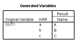
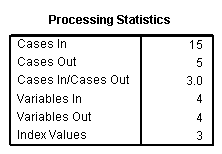
   TRIAL        A        B        C

    1.00    26.00    32.00    31.00
    2.00    32.00    36.00    33.00
    3.00    35.00    38.00    35.00
    4.00     6.00     2.00     5.00
    5.00     5.00     5.00     3.00

Number of cases read:  5    Number of cases listed:  5
For additional examples of reshaping data from long to wide using the casestovars command, please see SPSS Learning Module: Reshaping data from long to wide in versions 11 and up . For examples using the vector and aggregate commands, please see SPSS Learning Module: Reshaping data from long to wide .
6. Counting
The count command is useful if you have items from a questionnaire that are on a Likert scale (e.g., 1 to 5). It creates a new variable that contains the count of the number of occurrences of a value across a list of variables. In the example below, we count how many times the value "3" occurs for each subject for the variables listed (q1, q2 and q3).
get file 'd:data08_2.sav'.
count total = q1 to q3 (3).
exe.
list q1 to q3 total.
      Q1       Q2       Q3    TOTAL

    3.00     3.00      .       2.00
    2.00     2.00    -9.00      .00
    3.00     1.00     2.00     1.00
    4.00     1.00     2.00      .00
   -8.00     1.00     3.00     1.00
   -8.00     2.00     1.00      .00
    3.00    -9.00     4.00     1.00
    4.00     4.00     2.00      .00
    1.00     1.00     1.00      .00
    2.00    -9.00     3.00     1.00
    3.00     3.00     2.00     2.00
    3.00     1.00     1.00     1.00
   -9.00     4.00     4.00      .00
     .       2.00     4.00      .00
    2.00     3.00     1.00     1.00

Number of cases read:  15    Number of cases listed:  15
7. The show command
The show command is an extremely handy command that displays current settings in SPSS. There are about 60 subcommands that you can use with the show command. One of the them is all, but I don’t like to use that one because it gives so much output. Let’s look at some examples using the show command. You can type show license. to see which modules are installed and when your license expires (always a good thing to know).
show license.
< output purposely omitted>
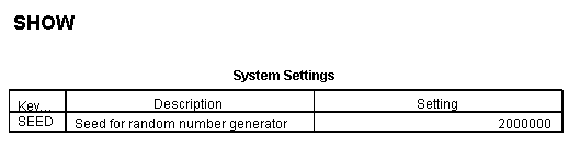
You can use the seed subcommand to see what seed is currently being used.
show seed.
Of course, you can list as many subcommands as you like on the show command.
show directory version n cache format.
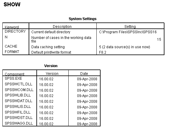
As we can see in the output above, the current default directory is "C:Program FilesSPSSIncSPSS16". There are 15 cases in the data set that is active. The "data cache setting" indicates that SPSS will cache the data set (save it) after five changes have been made. (The default is 20 changes.) We also see that the default print and write format is F8.2. This means that values will have eight spaces, including the decimal point, with two of the spaces after the decimal point. (In other words, five spaces before the decimal point, the decimal point, and two spaces after the decimal point, for a total of eight spaces.)
Information about the version of SPSS being used is given in the second table above. As you can see, the version is 16.0.2. The date at the right indicates when the .dll files were last updated. Another way to see which version of SPSS is being used is to click on Help -> About.
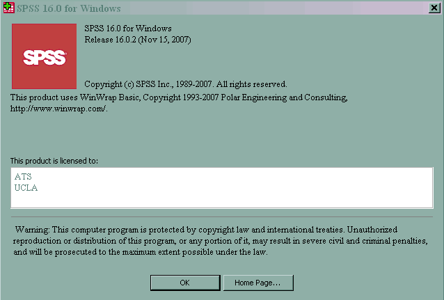
You may notice that the date is different than the one given above. The date given when you click on Show -> About references the file spssprod.inf for its information. The dates are not important; what is important is knowing exactly which version you are using so that you can determine if you are using the most up-to-date version, or if you need to look for patches to update SPSS. You want to have the latest patches for your version because the patches typically correct bugs in the program.
To check for updates from within SPSS, you can click on Help -> Check for Updates. Unfortunately, the updating feature in SPSS works better in some versions than in others, so you may be told that there are no updates (i.e., patches) when there actually are. You can visit Software Purchasing and Updating for information on the latest version and patches. More information can be found at Installing, Customizing and Updating SPSS .
Many of the values that we see with the show command can be changed with the set command.
compute f82 = 1.
set format=f8.6.
compute f86= 1.
exe.
list f82 f86.
     f82      f86

    1.00 1.000000
    1.00 1.000000
    1.00 1.000000
    1.00 1.000000
    1.00 1.000000
    1.00 1.000000
    1.00 1.000000
    1.00 1.000000
    1.00 1.000000
    1.00 1.000000
    1.00 1.000000
    1.00 1.000000
    1.00 1.000000
    1.00 1.000000
    1.00 1.000000

Number of cases read:  15    Number of cases listed:
Let’s return the format to its original setting.
set format = f8.2.
8. Active data sets and output files
SPSS allows users to have multiple data sets open at once. Users can also have multiple output files open at once. Not surprisingly, you control the data sets with the dataset commands and the output files with the output commands. You can use the dataset name command to name the active data set. You can then use that name when you want to manipulate that data set. For example, you can make a named data set active, you can close it, you can copy it, etc. These commands are particularly helpful when you want to copy variables, cases or variable properties from one data set to another.
/* dataset commands */
dataset activate.
dataset close.
dataset copy.
dataset declare.
dataset display.
dataset name.

/* output commands */
output activate.
output close.
output display.
output name.
output new.
output open.
output save.
In addition to controlling output files, you can control parts of the output from a procedure. This is done with the Output Management System, or OMS. OMS is particularly useful when you need to get one or more specific values from an output and use those in the next step of your analysis or program. For example, you may want to capture the regression coefficients from one model and use them with a different data set. You would need the oms and dataset commands to do this. We have some examples using the OMS commands at SPSS FAQ: How can I output my results to a data file in SPSS? and SPSS FAQ: How can I use aggregate and OMS to help explain a three-way interaction in ANOVA?
/* oms commands */
oms.
omsend.
omsinfo.
omslog.
9. More on saving files
We covered the save command back at the beginning of the Part 1 of the SPSS Syntax Seminar. Below, we look at some of the subcommands that are available with the command. Below are examples showing how to compress an SPSS data file and how to save only selected cases.
save outfile "D:mydata_compress.sav"
/compress.

filter by comp_flag.
save outfile "D:mydata_comp.sav"
/unselected = delete.

get file "D:mydata_comp.sav".

get file "d:data08_2.sav".
The save translate command is used to save a data file in a different format, such as Stata, SAS and .csv. Despite much wishful thinking, there is no command to translate SPSS syntax into SAS or Stata syntax. Sorry.
* saving a Stata 8 SE file.
save translate outfile = "D:mydata.dta"
/version = 8
/type = stata
/edition = se.

* saving a SAS file.
save translate outfile = "D:mydata.sas7bdat"
/valfile = "D:labels.sas"
/platform = windows
/type = sas
/version = 7
/replace.

* saving a comma separated file without variable names at the top.
* good for making Mplus data files.
save translate outfile = "D:mydata.csv"
/type = csv.

* csv file with names at the top and labels.
save translate outfile = "D:mydata.csv"
/type = csv
/fieldnames
/cells = labels.
10. Dates
Dates are simply numeric variables in SPSS. Because “Time 0” was a really long time ago, the numeric values of current dates in SPSS are extremely large. Dates are stored as the number of seconds from midnight, October 14, 1582 (the beginning of the Gregorian calendar). Therefore, you usually need to do some math in order to calculate the number of days (or months or years) between two dates. (Sometimes it is handy to know that there are 86,400 seconds in a day.) Because dates are stored as numbers, you can do standard mathematical operations on them, such as adding or subtracting them. If your date is displayed as stars or if only part of the year is showing in the SPSS Data Editor, you can make the column wider and the dates will display properly.
Because the topic of dates is such a large one, we are going to stop here. If you need to input or manipulate dates in your data set, please visit our pages on dates at SPSS Learning Module: Using dates in SPSS and SPSS Library: Inputting and manipulating dates in SPSS .
11. Other commands that we didn’t cover
As you might expect, there are many other really useful commands that we didn’t have time to cover. A partial list of these commands includes:
flip.
insert.
apply dictionary.
datafile attribute.
variable attribute.
update.
codebook. (new to SPSS version 17)
You can look in the SPSS Command Syntax Reference for more information on these commands. You can access the Command Syntax Reference by clicking on Help -> Command Syntax Reference from any of the SPSS windows.
12. Updating SPSS
To check for updates from within SPSS, you can click on Help -> Check for Updates. Unfortunately, the updating feature in SPSS works better in some versions than in others, so you may be told that there are no updates (i.e., patches) when there actually are. You can visit Software Purchasing and Updating for information on the latest version and patches. More information can be found at Installing, Customizing and Updating SPSS .