Introduction
Power analysis is the name given to the process for determining the sample size for a research study. The technical definition of power is the probability of detecting a "true" effect when it exists. Many students think that there is a simple formula for determining sample size for every research situation. However, the reality it that there are many research situations that are so complex that they almost defy rational power analysis. In most cases, power analysis involves making simplifying assumptions that make the problem tractable and running the analyses numerous times with different variations to cover all of the contingencies.
In this unit we will try to illustrate how to do a power analysis for a multiple regression model that has two control variables, one continuous research variable and one categorical research variable (three levels). We will be interested in the number of subjects we would require to detect the hypothesized effects of the research variables.
Description of the experiment
A school district is designing a multiple regression study looking at the effect of gender, family income, mother’s education and language spoken in the home on the English language proficiency scores of Latino high school students. The variables gender and family income are control variables and not of primary research interest. Mother’s education is a continuous research variable that measures the number of years that the mother attended school. The range of this variable is expected to be from 4 to 20. The variable language spoken in the home is a categorical research variable with three levels: 1) Spanish only, 2) both Spanish and English, and 3) English only. Since there are three levels, it will take two dummy variables to code language spoken in the home.
The full regression model will look something like this:
-
engprof = b0 + b1(gender) + b2(income) + b3(momeduc)
+ b4(homelang1) + b5(homelang2)
Thus, the primary research hypotheses are the test of b3 and the joint test of b4 and b5. These tests are equivalent to testing the change in R2 when momeduc (or homelang1 and homelang2) are added last to the regression equation.
The power analysis
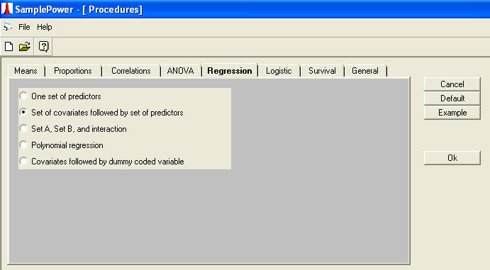
We will make use of the Sample Power procedure described as ‘Set of covariates followed by set of predictors’ under the ‘Regression’ tab in the Procedures catalog.
We believe, after looking through previous research, that the R2 for the full-model with five predictor variables (2 control, 1 continuous research, and 2 dummy variables for the categorical variable) will be will be about 0.48.
Let’s start with the continuous predictor (momeduc). We think that it will add about 0.03 to the R2 when it is added last to the model. This means that the R2 for the model without the variable (the reduced model) would be about 0.45, which leads to the difference in R2 (Increment to R2) of .03. The total number of variables is 5 (meaning 4 variables in the Covariates set) and the number being tested (Main set) is one. We will run the procedure for powers equal to .7, .8 and .9 by clicking the ‘Find N for any power’ button and adjusting the value accordingly.
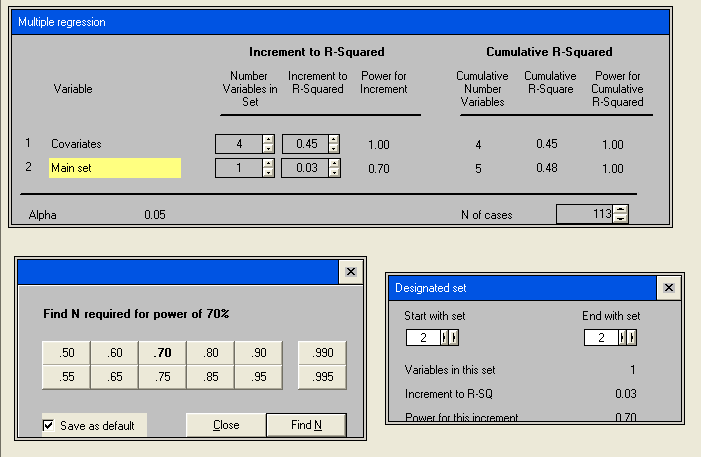

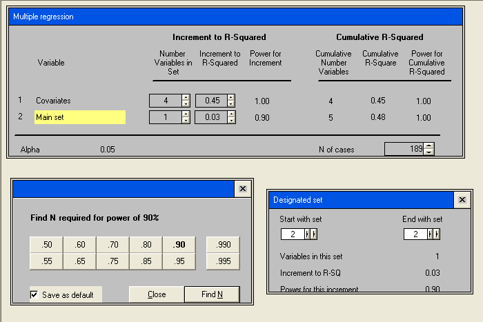
This gives us a set of sample sizes ranging from 113 to 189, depending on power.
Let’s see how this compares with the sample sizes required by the categorical predictor (homelang1 and homelang2) which uses two dummy variables in the model. We believe that the change in R2 attributed to the two dummy variables will be about 0.025. This would give an R2 of 0.455. The number of variables in the Covariates set stays at 4 while the number in the main set is now 2. To enter some of these new inputs, click on the ‘Decimals displayed’ button and increase the Decimals for R-Squared to 3.
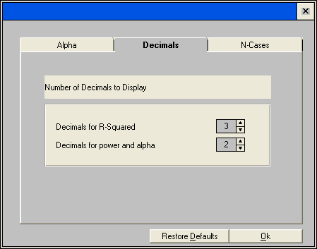
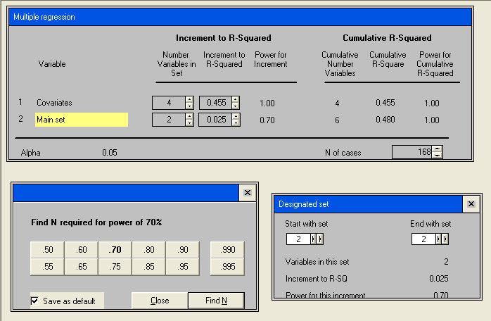


This series of power analyses yielded sample sizes ranging from 168 to 271. These sample sizes are larger than those of the continuous research variable.
If it is the case that both of these research variables are important, we might want to take into account that we are testing two separate hypotheses (one for the continuous and one for the categorical) by adjusting the alpha level. The simplest but most draconian method would be to use a Bonferroni adjustment by dividing the nominal alpha level, 0.05, by the number of hypotheses, 2, yielding an alpha of 0.025. We can adjust alpha in Sample Power by clicking on the current value and changing it.
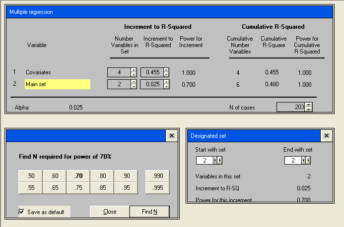
We will rerun the categorical variable power analysis using the new adjusted alpha level.
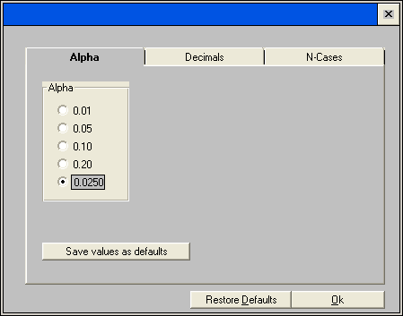
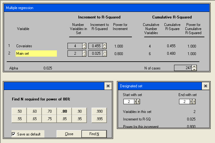
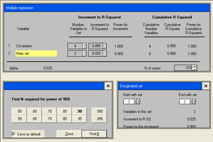
The Bonferroni adjustment assumes that the tests of the two hypotheses are independent, which is, in fact, not the case. The squared correlation between the two sets of predictors is about .2 which is equivalent to a correlation of approximately .45. Using an Internet applet to compute a Bonferroni adjusted alpha taking into account the correlation gives us an adjusted alpha value of 0.034 to use in the power analysis.
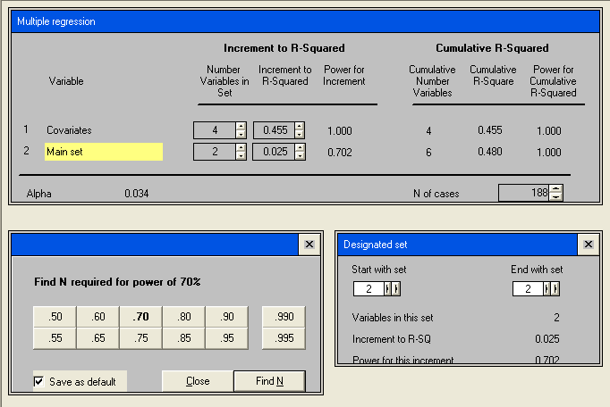
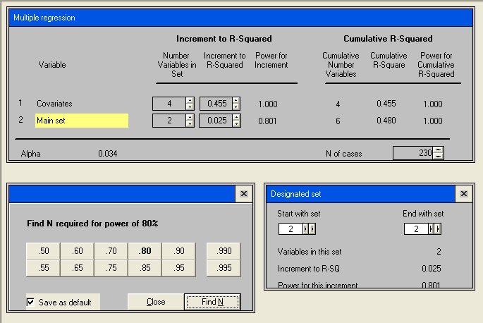
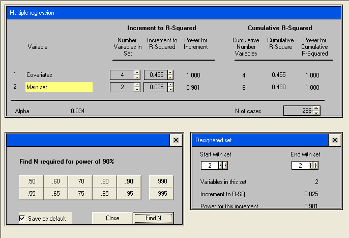
Based on this series of power analyses, the school district has decided to collect data on a sample of about 230 students. This sample size should yield a power of around 0.8 in testing hypotheses concerning both the continuous research variable (momeduc) and the categorical research variable (homelang1 and homelang2). The nominal alpha level is 0.05 but has been adjusted to .034 to take into account the number of hypotheses tested and the correlation between the predictors.
For more information on power analysis, please visit our Introduction to Power Analysis seminar.
