Examples
Example 1. A company markets an eight week long weight loss program and claims that at the end of the program on average a participant will have lost 5 pounds. On the other hand, you have studied the program and you believe that their program is scientifically unsound and shouldn’t work at all. With some limited funding at hand, you want test the hypothesis that the weight loss program does not help people lose weight. Your plan is to get a random sample of people and put them on the program. You will measure their weight at the beginning of the program and then measure their weight again at the end of the program. Based on some previous research, you believe that the standard deviation of their weight differences over eight weeks will be 5 pounds. You now want to know how many people you should enroll in the program to test your hypothesis.
Example 2. A human factors researcher wants to study the difference between dominant hand and the non-dominant hand in terms of manual dexterity. She designs an experiment where each subject would place 10 small beads on the table in a bowl, once with the dominant hand and once with the non-dominant hand. She measured the number seconds needed in each round to complete the task. She has also decided that the order in which the two hands are measured should be counter balanced. She expects that the average difference in time would be 5 seconds with the dominant hand being more efficient with standard deviation of 10. She collects her data on a sample of 35 subjects. The question is, what is the statistical power of her design with an N of 35 to detect the difference in the magnitude of 5 seconds?
Prelude to the power analysis
In both of the examples described above, there are two measures on each subject and we are interested in testing the mean of the difference of the two measures. This can be done with a t-test for paired samples (dependent samples). In a power analysis, there is always a pair of hypotheses: a specific null hypothesis and a specific alternative hypothesis. In Example 1, the null hypothesis is that the mean weight loss is 5 pounds and the alternative is that the weight loss is zero pounds. In Example 2, the null hypothesis is that mean difference is zero seconds and the alternative hypothesis is that the mean difference is 5 seconds.
Power is the probability of rejecting the null hypothesis when the specific alternative hypothesis is true. There are two different aspects of power analysis. One is to calculate the sample size necessary to achieve a specified power. The other aspect is to calculate the power achieved when given a specific sample size.
Both of these calculations depend on the Type I error rate, the significance level. The significance level (called alpha) is the probability of rejecting H0 when it is actually true. The smaller the Type I error rate, the larger the sample size required for the same power. Likewise, the smaller the Type I error rate, the smaller the power for the same sample size. This is the trade-off between the reliability and sensitivity of the test.
Power analysis
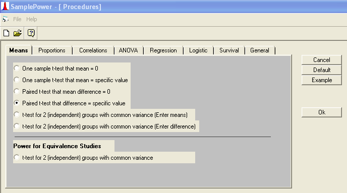
In Sample Power, it is fairly straightforward to perform a power analysis for the paired sample t-test. After opening the program and starting a new analysis, we simply select ‘Paired t-test that difference = specific value’ and click ‘Okay’. This opens up a table of inputs, allowing us to enter the mean difference (the mean for the alternative hypothesis) and test against the constant (mean for the null hypothesis). We will proceed using the situation described in Example 1.
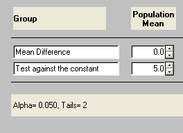
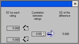
Assuming the standard deviation for the two groups is equal, we enter 5 for each in the standard deviation calculator (resembling a flowchart).
Following this, clicking on the icon bearing a set of binoculars and an arrow labeled ‘Find N for any power’ calls up a table of power values. Clicking the desired value (in our case, .85) followed by ‘Find N’ produces the wanted result.
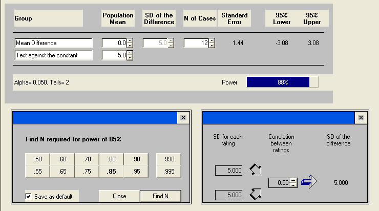
Twelve people are required to achieve .85 power with an alpha of .05.
Next, let’s change the level of significance to .01 with a power of .85, accomplished by clicking the alpha value in the lower left corner and inputting the new value. What does this mean for our sample size calculation? We click on Alpha, then the new value, and set the inputs.
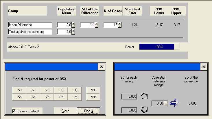
As you can see, the sample size goes up from 12 to 17 for specified power of .85 when alpha drops from .05 to .01. This means if we want our test to be more reliable, i.e., not rejecting the null hypothesis in case it is true, we will need a larger sample size. Remember all the calculation is under the normality assumption. If the distribution is not normal, then 17 subjects are, in general, not enough for this t-test.
Now, let’s now turn our calculation around the other way and calculate the power of an experiment given the number of subjects. Let’s look at Example 2. In this example, our researcher has already collected data on 35 subjects. How much statistical power does her design have to detect the difference of 5 seconds with standard deviation of 10 seconds?
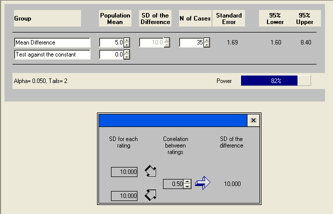
This means that the researcher would detect the difference of 5 seconds about 82 percent of the time. Notice we did this as two-sided test. But since it is believed that our dominant hand is always better than the non-dominant hand, the researcher actually could conduct a one-tailed test. Now, let’s recalculate the power for one-tailed paired-sample t-test. Clicking the number of tails in the lower-left corner allows it to be adjusted.
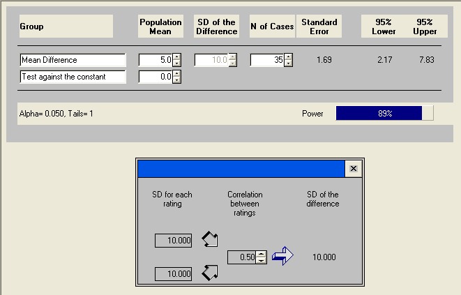
Recall that we set the correlation between the two measures at .5 for all the calculations we have done. Let’s take a look at how the strength of correlation affects the sample size.
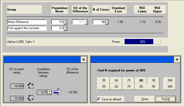
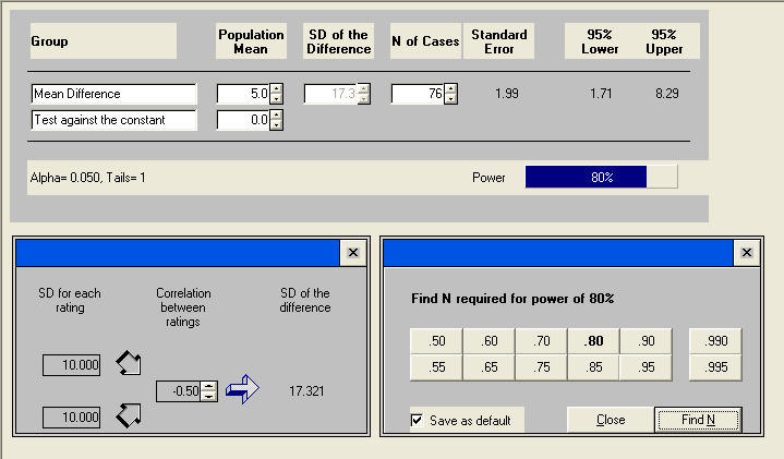
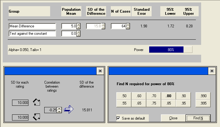
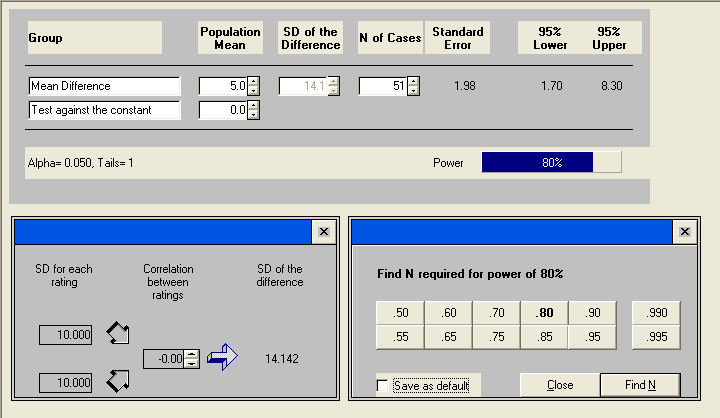

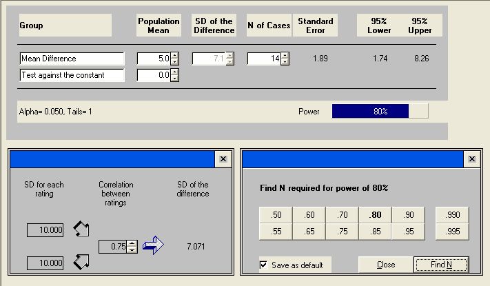
We can see clearly that the more positively correlated the two measures are, the smaller the sample size needs to be.
Discussion
An important technical assumption is the normality assumption. If the distribution is skewed, then a small sample size may not have the power shown in the results, because the value in the results is calculated using the method based on the normality assumption. It might not even be a good idea to do a t-test on a small sample to begin with.
What we really need to know is the difference between the two means, not the individual values. In fact, what really matters is the difference of the means over the standard deviation. We call this the effect size. It is usually not an easy task to determine the effect size before collecting data. It usually comes from studying the existing literature or from pilot studies. A good estimate of the effect size is the key to a successful power analysis.
For more information on power analysis, please visit our Introduction to Power Analysis seminar.
