Chapter Outline
    2.0 Regression Diagnostics
    2.1 Unusual and Influential data
    2.2 Tests on Normality of Residuals
    2.3 Tests on Nonconstant Error of Variance
    2.4 Tests on Multicollinearity
    2.5 Tests on Nonlinearity
    2.6 Model Specification
    2.7 Issues of Independence
    2.8 Summary
    2.9 For more information

2.0 Regression Diagnostics

In our last chapter, we learned how to do ordinary linear regression with SPSS, concluding with methods for examining the distribution of variables to check for non-normally distributed variables as a first look at checking assumptions in regression.  Without verifying that your data have met the regression assumptions, your results may be misleading.  This chapter will explore how you can use SPSS to test whether your data meet the assumptions of linear regression.  In particular, we will consider the following assumptions.

• Linearity – the relationships between the predictors and the outcome variable should be linear
• Normality – the errors should be normally distributed – technically normality is necessary only for the t-tests to be valid, estimation of the coefficients only requires that the errors be identically and independently distributed
• Homogeneity of variance (homoscedasticity) – the error variance should be constant
• Independence – the errors associated with one observation are not correlated with the errors of any other observation

• Model specification – the model should be properly specified (including all relevant variables, and excluding irrelevant variables)

Additionally, there are issues that can arise during the analysis that, while strictly speaking are not assumptions of regression, are none the less, of great concern to regression analysts.

• Influence – individual observations that exert undue influence on the coefficients
• Collinearity – predictors that are highly collinear, i.e. linearly related, can cause problems in estimating the regression coefficients.

Many graphical methods and numerical tests have been developed over the years for regression diagnostics and SPSS makes many of these methods easy to access and use. In this chapter, we will explore these methods and show how to verify regression assumptions and detect potential problems using SPSS.

2.1 Unusual and Influential data

A single observation that is substantially different from all other observations can make a large difference in the results of your regression analysis.  If a single observation (or small group of observations) substantially changes your results, you would want to know about this and investigate further.  There are three ways that an observation can be unusual.

Outliers: In linear regression, an outlier is an observation with large residual. In other words, it is an observation whose dependent-variable value is unusual given its values on the predictor variables. An outlier may indicate a sample peculiarity or may indicate a data entry error or other problem.

Leverage: An observation with an extreme value on a predictor variable is called a point with high leverage. Leverage is a measure of how far an observation deviates from the mean of that variable. These leverage points can have an unusually large effect on the estimate of regression coefficients.

Influence: An observation is said to be influential if removing the observation substantially changes the estimate of coefficients. Influence can be thought of as the product of leverage and outlierness.

How can we identify these three types of observations? Let’s look at an example dataset called crime. This dataset  appears in Statistical Methods for Social Sciences, Third Edition by Alan Agresti and Barbara Finlay (Prentice Hall, 1997). The variables are state id (sid), state name (state), violent crimes per 100,000 people (crime), murders per 1,000,000 (murder),  the percent of the population living in metropolitan areas (pctmetro), the percent of the population that is white (pctwhite), percent of population with a high school education or above (pcths), percent of population living under poverty line (poverty), and percent of population that are single parents (single).   Below we read in the file and do some descriptive statistics on these variables.  You can click crime.sav to access this file, or see the Regression with SPSS page to download all of the data files used in this book.

get file = "c:spssregcrime.sav".

descriptives
  /var=crime murder pctmetro pctwhite pcths poverty single.

 

Descriptive Statistics

	N	Minimum	Maximum	Mean	Std. Deviation
CRIME	51	82	2922	612.84	441.100
MURDER	51	1.60	78.50	8.7275	10.71758
PCTMETRO	51	24.00	100.00	67.3902	21.95713
PCTWHITE	51	31.80	98.50	84.1157	13.25839
PCTHS	51	64.30	86.60	76.2235	5.59209
POVERTY	51	8.00	26.40	14.2588	4.58424
SINGLE	51	8.40	22.10	11.3255	2.12149
Valid N (listwise)	51

Let’s say that we want to predict crime by pctmetro, poverty, and single . That is to say, we want to build a linear regression model between the response variable crime and the independent variables pctmetro, poverty and single. We will first look at the scatter plots of crime against each of the predictor variables before the regression analysis so we will have some ideas about potential problems. We can create a scatterplot matrix of these variables as shown below.

graph
  /scatterplot(matrix)=crime murder pctmetro pctwhite pcths poverty single .

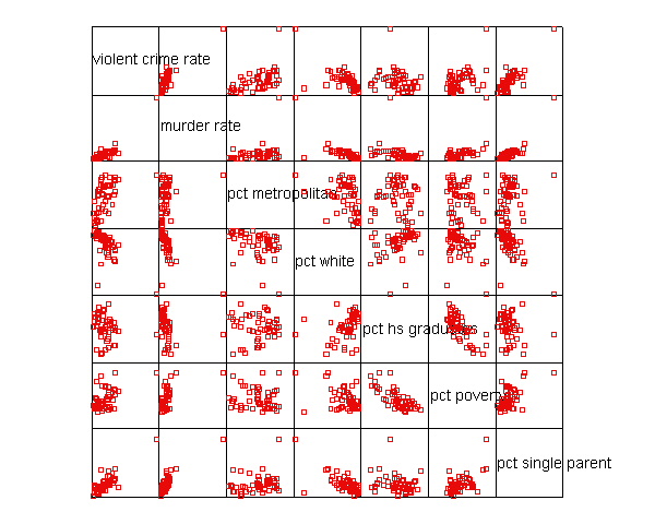
The graphs of crime with other variables show some potential problems.  In every plot, we see a data point that is far away from the rest of the data points. Let’s make individual graphs of crime with pctmetro and poverty and single so we can get a better view of these scatterplots.  We will use BY state(name) to plot the state name instead of a point.

GRAPH /SCATTERPLOT(BIVAR)=pctmetro WITH crime BY state(name) .

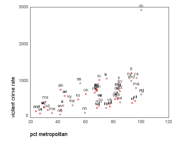
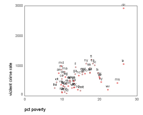
GRAPH /SCATTERPLOT(BIVAR)=poverty WITH crime BY state(name) .

GRAPH /SCATTERPLOT(BIVAR)=single WITH crime BY state(name) .

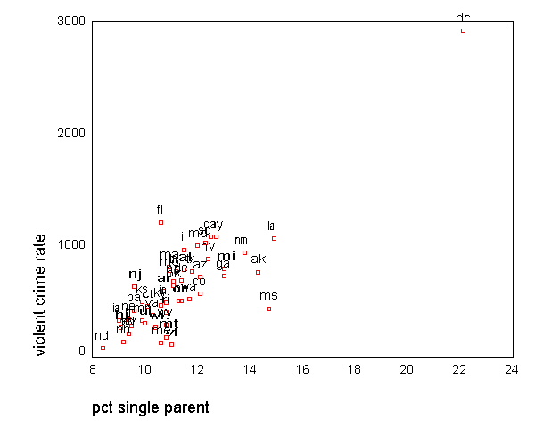
All the scatter plots suggest that the observation for state = "dc" is a point that requires extra attention since it stands out away from all of the other points. We will keep it in mind when we do our regression analysis.

Now let's try the regression command predicting crime from pctmetro poverty and single.  We will go step-by-step to identify all the potentially unusual or influential points afterwards. 

regression
  /dependent crime
  /method=enter pctmetro poverty single.
 

Variables Entered/Removed(b)

Model	Variables Entered	Variables Removed	Method
1	SINGLE, PCTMETRO, POVERTY(a)	.	Enter
a All requested variables entered.
b Dependent Variable: CRIME




Model Summary(b)

Model	R	R Square	Adjusted R Square	Std. Error of the Estimate
1	.916(a)	.840	.830	182.068
a Predictors: (Constant), SINGLE, PCTMETRO, POVERTY
b Dependent Variable: CRIME




ANOVA(b)

Model		Sum of Squares	df	Mean Square	F	Sig.
1	Regression	8170480.211	3	2723493.404	82.160	.000(a)
	Residual	1557994.534	47	33148.820
	Total	9728474.745	50
a Predictors: (Constant), SINGLE, PCTMETRO, POVERTY
b Dependent Variable: CRIME






Coefficients(a)

		Unstandardized Coefficients		Standardized Coefficients	t	Sig.
Model		B	Std. Error	Beta
1	(Constant)	-1666.436	147.852		-11.271	.000
	PCTMETRO	7.829	1.255	.390	6.240	.000
	POVERTY	17.680	6.941	.184	2.547	.014
	SINGLE	132.408	15.503	.637	8.541	.000
a Dependent Variable: CRIME

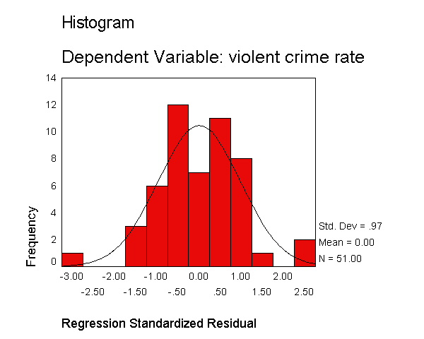
Let's examine the standardized residuals as a first means for identifying outliers. Below we use the /residuals=histogram subcommand to request a histogram for the standardized residuals.  As you see, we get the standard output that we got above, as well as a table with information about the smallest and largest residuals, and a histogram of the standardized residuals.  The histogram indicates a couple of extreme residuals worthy of investigation.

regression
  /dependent crime
  /method=enter pctmetro poverty single
  /residuals=histogram.

Variables Entered/Removed(b)

Model	Variables Entered	Variables Removed	Method
1	SINGLE, PCTMETRO, POVERTY(a)	.	Enter
a All requested variables entered.
b Dependent Variable: CRIME

Model Summary(b)

Model	R	R Square	Adjusted R Square	Std. Error of the Estimate
1	.916(a)	.840	.830	182.068
a Predictors: (Constant), SINGLE, PCTMETRO, POVERTY
b Dependent Variable: CRIME

ANOVA(b)

Model		Sum of Squares	df	Mean Square	F	Sig.
1	Regression	8170480.211	3	2723493.404	82.160	.000(a)
	Residual	1557994.534	47	33148.820
	Total	9728474.745	50
a Predictors: (Constant), SINGLE, PCTMETRO, POVERTY
b Dependent Variable: CRIME

Coefficients(a)

		Unstandardized Coefficients		Standardized Coefficients	t	Sig.
Model		B	Std. Error	Beta
1	(Constant)	-1666.436	147.852		-11.271	.000
	PCTMETRO	7.829	1.255	.390	6.240	.000
	POVERTY	17.680	6.941	.184	2.547	.014
	SINGLE	132.408	15.503	.637	8.541	.000
a Dependent Variable: CRIME

Residuals Statistics(a)

	Minimum	Maximum	Mean	Std. Deviation	N
Predicted Value	-30.51	2509.43	612.84	404.240	51
Residual	-523.01	426.11	.00	176.522	51
Std. Predicted Value	-1.592	4.692	.000	1.000	51
Std. Residual	-2.873	2.340	.000	.970	51
a Dependent Variable: CRIME

regression
  /dependent crime
  /method=enter pctmetro poverty single
  /residuals=histogram(sdresid).

Residuals Statistics(a)

	Minimum	Maximum	Mean	Std. Deviation	N
Predicted Value	-30.51	2509.43	612.84	404.240	51
Std. Predicted Value	-1.592	4.692	.000	1.000	51
Standard Error of Predicted Value	25.788	133.343	47.561	18.563	51
Adjusted Predicted Value	-39.26	2032.11	605.66	369.075	51
Residual	-523.01	426.11	.00	176.522	51
Std. Residual	-2.873	2.340	.000	.970	51
Stud. Residual	-3.194	3.328	.015	1.072	51
Deleted Residual	-646.50	889.89	7.18	223.668	51
Stud. Deleted Residual	-3.571	3.766	.018	1.133	51
Mahal. Distance	.023	25.839	2.941	4.014	51
Cook's Distance	.000	3.203	.089	.454	51
Centered Leverage Value	.000	.517	.059	.080	51
a Dependent Variable: CRIME

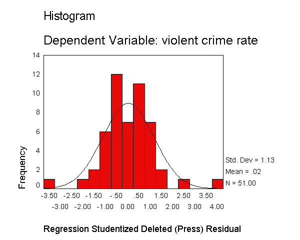
The histogram shows some possible outliers.  We can use the outliers(sdresid) and id(state) options to request the 10 most extreme values for the studentized deleted residual to be displayed labeled by the state from which the observation originated.  Below we show the output generated by this option, omitting all of the rest of the output to save space.  You can see that "dc" has the largest value (3.766) followed by "ms" (-3.571) and "fl" (2.620).

regression
  /dependent crime
  /method=enter pctmetro poverty single
  /residuals=histogram(sdresid) id(state) outliers(sdresid).

Outlier Statistics(a)

		Case Number	STATE	Statistic
Stud. Deleted Residual	1	51	dc	3.766
	2	25	ms	-3.571
	3	9	fl	2.620
	4	18	la	-1.839
	5	39	ri	-1.686
	6	12	ia	1.590
	7	47	wa	-1.304
	8	13	id	1.293
	9	14	il	1.152
	10	35	oh	-1.148
a Dependent Variable: CRIME

We can use the /casewise subcommand below to request a display of all observations where the sdresid exceeds 2.  To save space, we show just the new output generated by the /casewise subcommand. This shows us that Florida, Mississippi and Washington DC have sdresid values exceeding 2.

regression
  /dependent crime
  /method=enter pctmetro poverty single
  /residuals=histogram(sdresid) id(state) outliers(sdresid)
  /casewise=plot(sdresid) outliers(2)  .

Casewise Diagnostics(a)

Case Number	STATE	Stud. Deleted Residual	CRIME	Predicted Value	Residual
9	fl	2.620	1206	779.89	426.11
25	ms	-3.571	434	957.01	-523.01
51	dc	3.766	2922	2509.43	412.57
a Dependent Variable: CRIME

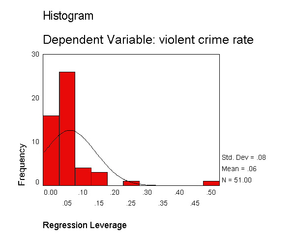
Now let's look at the leverage values to identify observations that will have potential great influence on regression coefficient estimates.  We can include lever with the histogram( )  and the outliers( ) options to get more information about observations with high leverage.  We show just the new output generated by these additional subcommands below.  Generally, a point with leverage greater than (2k+2)/n should be carefully examined. Here k is the number of predictors and n is the number of observations, so a value exceeding (2*3+2)/51 = .1568 would be worthy of further investigation.  As you see, there are 4 observations that have leverage values higher than .1568.

regression
  /dependent crime
  /method=enter pctmetro poverty single
  /residuals=histogram(sdresid lever) id(state) outliers(sdresid lever)
  /casewise=plot(sdresid) outliers(2).

Outlier Statistics(a)

		Case Number	STATE	Statistic
Stud. Deleted Residual	1	51	dc	3.766
	2	25	ms	-3.571
	3	9	fl	2.620
	4	18	la	-1.839
	5	39	ri	-1.686
	6	12	ia	1.590
	7	47	wa	-1.304
	8	13	id	1.293
	9	14	il	1.152
	10	35	oh	-1.148
Centered Leverage Value	1	51	dc	.517
	2	1	ak	.241
	3	25	ms	.171
	4	49	wv	.161
	5	18	la	.146
	6	46	vt	.117
	7	9	fl	.083
	8	26	mt	.080
	9	31	nj	.075
	10	17	ky	.072
a Dependent Variable: CRIME

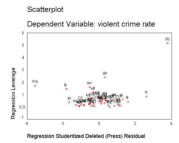
As we have seen, DC is an observation that both has a large residual and large leverage.  Such points are potentially the most influential.  We can make a plot that shows the leverage by the residual and look for observations that are high in leverage and have a high residual.  We can do this using the /scatterplot subcommand as shown below.  This is a quick way of checking potential influential observations and outliers at the same time. Both types of points are of great concern for us.  As we see, "dc" is both a high residual and high leverage point, and "ms" has an extremely negative residual but does not have such a high leverage.

regression
  /dependent crime
  /method=enter pctmetro poverty single
  /residuals=histogram(sdresid lever) id(state) outliers(sdresid, lever)
  /casewise=plot(sdresid)  outliers(2)
  /scatterplot(*lever, *sdresid).

Now let's move on to overall measures of influence, specifically let's look at Cook's D, which combines information on the residual and leverage. The lowest value that Cook's D can assume is zero, and the higher the Cook's D is, the more influential the point is. The conventional cut-off point is 4/n, or in this case 4/51 or .078. Below we add the cook keyword to the outliers( ) option and also on the /casewise subcommand and below we see that for the 3 outliers flagged in the "Casewise Diagnostics" table, the value of Cook's D exceeds this cutoff.  And, in the "Outlier Statistics" table, we see that "dc", "ms", "fl" and "la" are the 4 states that exceed this cutoff, all others falling below this threshold.

regression
  /dependent crime
  /method=enter pctmetro poverty single
  /residuals=histogram(sdresid lever) id(state) outliers(sdresid, lever, cook)
  /casewise=plot(sdresid)  outliers(2) cook dffit
  /scatterplot(*lever, *sdresid).

Casewise Diagnostics(a)

Case Number	STATE	Stud. Deleted Residual	CRIME	Cook's Distance	DFFIT
9	fl	2.620	1206	.174	48.507
25	ms	-3.571	434	.602	-123.490
51	dc	3.766	2922	3.203	477.319
a Dependent Variable: CRIME

Outlier Statistics(a)

		Case Number	STATE	Statistic	Sig. F
Stud. Deleted Residual	1	51	dc	3.766
	2	25	ms	-3.571
	3	9	fl	2.620
	4	18	la	-1.839
	5	39	ri	-1.686
	6	12	ia	1.590
	7	47	wa	-1.304
	8	13	id	1.293
	9	14	il	1.152
	10	35	oh	-1.148
Cook's Distance	1	51	dc	3.203	.021
	2	25	ms	.602	.663
	3	9	fl	.174	.951
	4	18	la	.159	.958
	5	39	ri	.041	.997
	6	12	ia	.041	.997
	7	13	id	.037	.997
	8	20	md	.020	.999
	9	6	co	.018	.999
	10	49	wv	.016	.999
Centered Leverage Value	1	51	dc	.517
	2	1	ak	.241
	3	25	ms	.171
	4	49	wv	.161
	5	18	la	.146
	6	46	vt	.117
	7	9	fl	.083
	8	26	mt	.080
	9	31	nj	.075
	10	17	ky	.072
a Dependent Variable: CRIME

Cook's D can be thought of as a general measure of influence.  You can also consider more specific measures of influence that assess how each coefficient is changed by including the observation. Imagine that you compute the regression coefficients for the regression model with a particular case excluded, then recompute the model with the case included, and you observe the change in the regression coefficients due to including that case in the model.  This measure is called DFBETA and a DFBETA value can be computed for each observation for each predictor. As shown below, we use the /save sdbeta(sdbf) subcommand to save the DFBETA values for each of the predictors. This saves 4 variables into the current data file, sdfb1, sdfb2, sdfb3 and sdfb4, corresponding to the DFBETA for the Intercept and for pctmetro, poverty and for single, respectively.  We could replace sdfb with anything we like, and the variables created would start with the prefix that we provide.

regression
  /dependent crime
  /method=enter pctmetro poverty single
  /residuals=histogram(sdresid lever) id(state) outliers(sdresid, lever, cook)
  /casewise=plot(sdresid)  outliers(2) cook dffit
  /scatterplot(*lever, *sdresid)
  /save sdbeta(sdfb).

The /save sdbeta(sdfb) subcommand does not produce any new output, but we can see the variables it created for the first 10 cases using the list command below.  For example, by including the case for "ak" in the regression analysis (as compared to excluding this case), the coefficient for pctmetro would decrease by -.106 standard errors.  Likewise, by including the case for "ak" the coefficient for poverty decreases by -.131 standard errors, and the coefficient for single increases by .145 standard errors (as compared to a model excluding "ak"). Since the inclusion of an observation could either contribute to an increase or decrease in a regression coefficient, DFBETAs can be either positive or negative.  A DFBETA value in excess of  2/sqrt(n) merits further investigation. In this example, we would be concerned about absolute values in excess of 2/sqrt(51) or .28.

list
  /variables state sdfb1 sdfb2 sdfb3
  /cases from 1 to 10.

STATE       SDFB1       SDFB2       SDFB3

ak        -.10618     -.13134      .14518
al         .01243      .05529     -.02751
ar        -.06875      .17535     -.10526
az        -.09476     -.03088      .00124
ca         .01264      .00880     -.00364
co        -.03705      .19393     -.13846
ct        -.12016      .07446      .03017
de         .00558     -.01143      .00519
fl         .64175      .59593     -.56060
ga         .03171      .06426     -.09120

Number of cases read:  10    Number of cases listed:  10

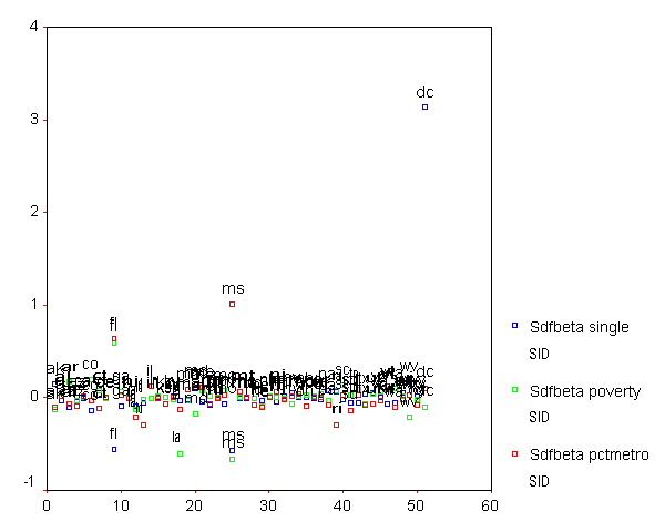
We can plot all three DFBETA values for the 3 coefficients against the state id in one graph shown below to help us see potentially troublesome observations.  We see changed the value labels for sdfb1 sdfb2 and sdfb3 so they would be shorter and more clearly labeled in the graph.  We can see that the DFBETA for single for "dc" is about 3, indicating that by including "dc" in the regression model, the coefficient for single is 3 standard errors larger than it would have been if "dc" had been omitted.  This is yet another bit of evidence that the observation for "dc" is very problematic.

VARIABLE LABLES sdfb1 "Sdfbeta pctmetro"
                              /sdfb2 "Sdfbeta poverty"
                              /sdfb3 "Sdfbeta single" .

GRAPH
  /SCATTERPLOT(OVERLAY)=sid sid sid  WITH sdfb1 sdfb2 sdfb3 (PAIR) BY state(name)
  /MISSING=LISTWISE .

The following table summarizes the general rules of thumb we use for the measures we have discussed for identifying observations worthy of further investigation (where k is the number of predictors and n is the number of observations).

We have shown a few examples of the variables that you can refer to in the /residuals  , /casewise,  /scatterplot and /save sdbeta(  ) subcommands. Here is a list of all of the variables that can be used on these subcommands; however, not all variables can be used on each subcommand.

PRED	Unstandardized predicted values.
RESID	Unstandardized residuals.
DRESID	Deleted residuals.
ADJPRED	Adjusted predicted values.
ZPRED	Standardized predicted values.
ZRESID	Standardized residuals.
SRESID	Studentized residuals.
SDRESID	Studentized deleted residuals.
SEPRED	Standard errors of the predicted values.
MAHAL	Mahalanobis distances.
COOK	Cook s distances.
LEVER	Centered leverage values.
DFBETA	Change in the regression coefficient that results from the deletion of the ith case. A DFBETA value is computed for each case for each regression coefficient generated by a model.
SDBETA	Standardized DFBETA. An SDBETA value is computed for each case for each regression coefficient generated by a model.
DFFIT	Change in the predicted value when the ith case is deleted.
SDFIT	Standardized DFFIT.
COVRATIO	Ratio of the determinant of the covariance matrix with the ith case deleted to the determinant of the covariance matrix with all cases included.
MCIN	Lower and upper bounds for the prediction interval of the mean predicted response. A lowerbound LMCIN and an upperbound UMCIN are generated. The default confidence interval is 95%. The confidence interval can be reset with the CIN subcommand. (See Dillon & Goldstein
ICIN	Lower and upper bounds for the prediction interval for a single observation. A lowerbound LICIN and an upperbound UICIN are generated. The default confidence interval is 95%. The confidence interval can be reset with the CIN subcommand. (See Dillon & Goldstein

regression
  /dependent crime
  /method=enter pctmetro poverty single.

<some output omitted to save space>





Coefficients(a)

		Unstandardized Coefficients		Standardized Coefficients	t	Sig.
Model		B	Std. Error	Beta
1	(Constant)	-1666.436	147.852		-11.271	.000
	PCTMETRO	7.829	1.255	.390	6.240	.000
	POVERTY	17.680	6.941	.184	2.547	.014
	SINGLE	132.408	15.503	.637	8.541	.000
a Dependent Variable: CRIME

Now, let's run the analysis omitting DC by using the filter command to omit "dc" from the analysis.  As we expect, deleting DC made a large change in the coefficient for single .The coefficient for single dropped from 132.4 to 89.4.  After having deleted DC, we would repeat the process we have illustrated in this section to search for any other outlying and influential observations.

compute filtvar = (state NE "dc").
filter by filtvar.
regression
  /dependent crime
  /method=enter pctmetro poverty single . 

<some output omitted to save space>

Coefficients(a)

		Unstandardized Coefficients		Standardized Coefficients	t	Sig.
Model		B	Std. Error	Beta
1	(Constant)	-1197.538	180.487		-6.635	.000
	PCTMETRO	7.712	1.109	.565	6.953	.000
	POVERTY	18.283	6.136	.265	2.980	.005
	SINGLE	89.401	17.836	.446	5.012	.000
a Dependent Variable: CRIME

Summary  

In this section, we explored a number of methods of identifying outliers and influential points. In a typical analysis, you would probably use only some of these methods. Generally speaking, there are two types of methods for assessing outliers: statistics such as residuals, leverage, and Cook's D, that assess the overall impact of an observation on the regression results, and statistics such as DFBETA that assess the specific impact of an observation on the regression coefficients. In our example, we found out that  DC was a point of major concern. We performed a regression with it and without it and the regression equations were very different. We can justify removing it from our analysis by reasoning that our model is to predict crime rate for states not for metropolitan areas.

2.2 Tests for Normality of Residuals

One of the assumptions of linear regression analysis is that the residuals are normally distributed. It is important to meet this assumption for the p-values for the t-tests to be valid. Let's use the elemapi2 data file we saw in Chapter 1 for these analyses.   Let's predict academic performance (api00) from percent receiving free meals (meals), percent of English language learners (ell), and percent of teachers with emergency credentials (emer).  We then use the /save command to generate residuals.

get file="c:spssregelemapi2.sav".
regression
  /dependent api00
  /method=enter meals ell emer
  /save resid(apires).

Variables Entered/Removed(b)

Model	Variables Entered	Variables Removed	Method
1	EMER, ELL, MEALS(a)	.	Enter
a All requested variables entered.
b Dependent Variable: API00




Model Summary(b)

Model	R	R Square	Adjusted R Square	Std. Error of the Estimate
1	.914(a)	.836	.835	57.820
a Predictors: (Constant), EMER, ELL, MEALS
b Dependent Variable: API00




ANOVA(b)

Model		Sum of Squares	df	Mean Square	F	Sig.
1	Regression	6749782.747	3	2249927.582	672.995	.000(a)
	Residual	1323889.251	396	3343.155
	Total	8073671.997	399
a Predictors: (Constant), EMER, ELL, MEALS
b Dependent Variable: API00







Coefficients(a)

		Unstandardized Coefficients		Standardized Coefficients	t	Sig.
Model		B	Std. Error	Beta
1	(Constant)	886.703	6.260		141.651	.000
	MEALS	-3.159	.150	-.709	-21.098	.000
	ELL	-.910	.185	-.159	-4.928	.000
	EMER	-1.573	.293	-.130	-5.368	.000
a Dependent Variable: API00




Casewise Diagnostics(a)

Case Number	Std. Residual	API00
93	3.087	604
226	-3.208	386
a Dependent Variable: API00




Residuals Statistics(a)

	Minimum	Maximum	Mean	Std. Deviation	N
Predicted Value	425.52	884.88	647.62	130.064	400
Residual	-185.47	178.48	.00	57.602	400
Std. Predicted Value	-1.708	1.824	.000	1.000	400
Std. Residual	-3.208	3.087	.000	.996	400
a Dependent Variable: API00

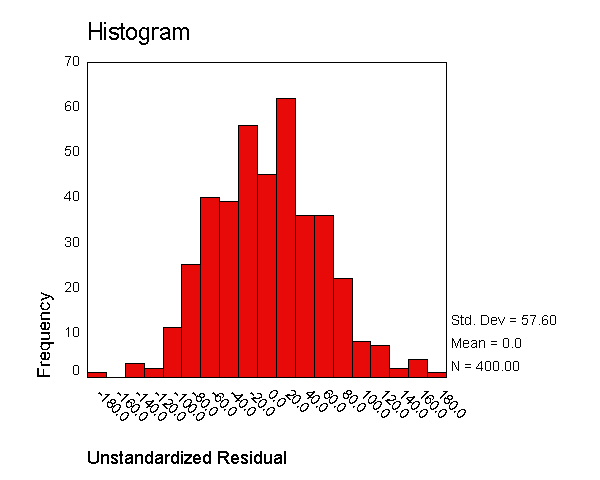
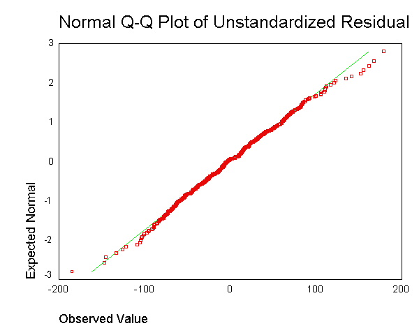
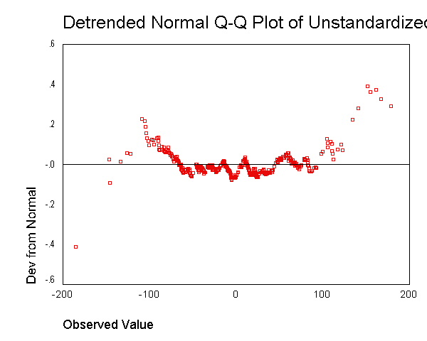
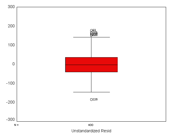
We now use the examine command to look at the normality of these residuals. All of the results from the examine command suggest that the residuals are normally distributed -- the skewness and kurtosis are near 0, the "tests of normality" are not significant, the histogram looks normal, and the Q-Q plot looks normal.  Based on these results, the residuals from this regression appear to conform to the assumption of being normally distributed.

examine
  variables=apires
  /plot boxplot stemleaf histogram npplot.

Case Processing Summary

	Cases
	Valid		Missing		Total
	N	Percent	N	Percent	N	Percent
APIRES	400	100.0%	0	.0%	400	100.0%




Descriptives

			Statistic	Std. Error
APIRES	Mean		.0000000	2.88011205
	95% Confidence Interval for Mean	Lower Bound	-5.6620909
		Upper Bound	5.6620909
	5% Trimmed Mean		-.7827765
	Median		-3.6572906
	Variance		3318.018
	Std. Deviation		57.60224104
	Minimum		-185.47331
	Maximum		178.48224
	Range		363.95555
	Interquartile Range		76.5523053
	Skewness		.171	.122
	Kurtosis		.135	.243




Tests of Normality

	Kolmogorov-Smirnov(a)			Shapiro-Wilk
	Statistic	df	Sig.	Statistic	df	Sig.
APIRES	.033	400	.200(*)	.996	400	.510
* This is a lower bound of the true significance.
a Lilliefors Significance Correction

Unstandardized Residual Stem-and-Leaf Plot

 Frequency    Stem &  Leaf
     1.00 Extremes    (=<-185)
     2.00       -1 .  4
     3.00       -1 .  2&
     7.00       -1 .  000
    15.00       -0 .  8888899
    35.00       -0 .  66666666667777777
    37.00       -0 .  444444444555555555
    49.00       -0 .  222222222222223333333333
    61.00       -0 .  000000000000000011111111111111
    48.00        0 .  000000111111111111111111
    49.00        0 .  222222222222233333333333
    28.00        0 .  4444445555555
    31.00        0 .  666666666677777
    16.00        0 .  88888899
     9.00        1 .  0011
     3.00        1 .  2&
     1.00        1 .  &
     5.00 Extremes    (>=152)
 Stem width:  100.0000
 Each leaf:       2 case(s)
 & denotes fractional leaves.

2.3 Heteroscedasticity

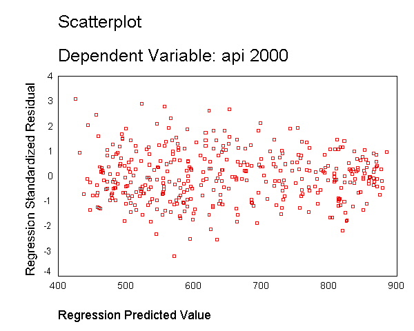
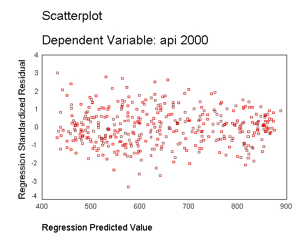
Another assumption of ordinary least squares regression is that the variance of the residuals is homogeneous across levels of the predicted values, also known as homoscedasticity. If the model is well-fitted, there should be no pattern to the residuals plotted against the fitted values. If the variance of the residuals is non-constant then the residual variance is said to be "heteroscedastic." Below we illustrate graphical methods for detecting heteroscedasticity. A commonly used graphical method is to use the residual versus fitted plot to show the residuals versus fitted (predicted) values.  Below we use the /scatterplot subcommand to plot *zresid (standardized residuals) by *pred (the predicted values).  We see that the pattern of the data points is getting a little narrower towards the right end, an indication of mild heteroscedasticity.

regression
  /dependent api00
  /method=enter meals ell emer
  /scatterplot(*zresid *pred).

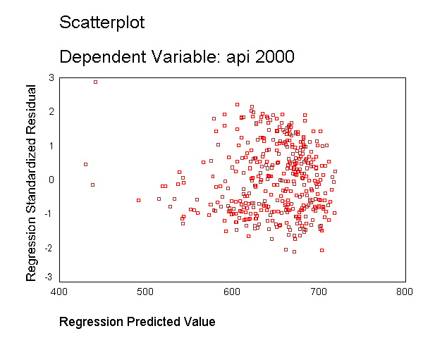
Let's run a model where we include just enroll as a predictor and show the residual vs. predicted plot.  As you can see, this plot shows serious heteroscedasticity.  The variability of the residuals when the predicted value is around 700 is much larger than when the predicted value is 600 or when the predicted value is 500.

regression
  /dependent api00
  /method=enter enroll
  /scatterplot(*zresid *pred).

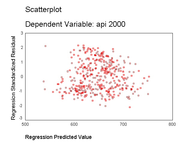
As we saw in Chapter 1, the variable enroll was skewed considerably to the right, and we found that by taking a log transformation, the transformed variable was more normally distributed. Below we transform enroll, run the regression and show the residual versus fitted plot. The distribution of the residuals is much improved.  Certainly, this is not a perfect distribution of residuals, but it is much better than the distribution with the untransformed variable.

compute lenroll = ln(enroll).
regression
  /dependent api00
  /method=enter lenroll
  /scatterplot(*zresid *pred).

Variables Entered/Removed(b)

Model	Variables Entered	Variables Removed	Method
1	LENROLL(a)	.	Enter
a All requested variables entered.
b Dependent Variable: API00




Model Summary(b)

Model	R	R Square	Adjusted R Square	Std. Error of the Estimate
1	.275(a)	.075	.073	136.946
a Predictors: (Constant), LENROLL
b Dependent Variable: API00




ANOVA(b)

Model		Sum of Squares	df	Mean Square	F	Sig.
1	Regression	609460.408	1	609460.408	32.497	.000(a)
	Residual	7464211.589	398	18754.300
	Total	8073671.997	399
a Predictors: (Constant), LENROLL
b Dependent Variable: API00






Coefficients(a)

		Unstandardized Coefficients		Standardized Coefficients	t	Sig.
Model		B	Std. Error	Beta
1	(Constant)	1170.429	91.966		12.727	.000
	LENROLL	-86.000	15.086	-.275	-5.701	.000
a Dependent Variable: API00




Residuals Statistics(a)

	Minimum	Maximum	Mean	Std. Deviation	N
Predicted Value	537.57	751.82	647.62	39.083	400
Residual	-288.65	295.47	.00	136.775	400
Std. Predicted Value	-2.816	2.666	.000	1.000	400
Std. Residual	-2.108	2.158	.000	.999	400
a Dependent Variable: API00

 

Finally, let's revisit the model we used at the start of this section, predicting api00 from meals, ell and emer.  Using this model, the distribution of the residuals looked very nice and even across the fitted values.   What if we add enroll to this model.  Will this automatically ruin the distribution of the residuals?  Let's add it and see.

regression
  /dependent api00
  /method=enter meals ell emer enroll
  /scatterplot(*zresid *pred).

Variables Entered/Removed(b)

Model	Variables Entered	Variables Removed	Method
1	ENROLL, MEALS, EMER, ELL(a)	.	Enter
a All requested variables entered.
b Dependent Variable: API00




Model Summary(b)

Model	R	R Square	Adjusted R Square	Std. Error of the Estimate
1	.915(a)	.838	.836	57.552
a Predictors: (Constant), ENROLL, MEALS, EMER, ELL
b Dependent Variable: API00




ANOVA(b)

Model		Sum of Squares	df	Mean Square	F	Sig.
1	Regression	6765344.050	4	1691336.012	510.635	.000(a)
	Residual	1308327.948	395	3312.223
	Total	8073671.997	399
a Predictors: (Constant), ENROLL, MEALS, EMER, ELL
b Dependent Variable: API00






Coefficients(a)

		Unstandardized Coefficients		Standardized Coefficients	t	Sig.
Model		B	Std. Error	Beta
1	(Constant)	899.147	8.472		106.128	.000
	MEALS	-3.222	.152	-.723	-21.223	.000
	ELL	-.768	.195	-.134	-3.934	.000
	EMER	-1.418	.300	-.117	-4.721	.000
	ENROLL	-3.126E-02	.014	-.050	-2.168	.031
a Dependent Variable: API00




Casewise Diagnostics(a)

Case Number	Std. Residual	API00
93	3.004	604
226	-3.311	386
a Dependent Variable: API00




Residuals Statistics(a)

	Minimum	Maximum	Mean	Std. Deviation	N
Predicted Value	430.82	888.08	647.62	130.214	400
Residual	-190.56	172.86	.00	57.263	400
Std. Predicted Value	-1.665	1.847	.000	1.000	400
Std. Residual	-3.311	3.004	.000	.995	400
a Dependent Variable: API00

 

As you can see, the distribution of the residuals looks fine, even after we added the variable enroll. When we had just the variable enroll in the model, we did a log transformation to improve the distribution of the residuals, but when enroll was part of a model with other variables, the residuals looked good so no transformation was needed.  This illustrates how the distribution of the residuals, not the distribution of the predictor, was the guiding factor in determining whether a transformation was needed.

2.4 Collinearity

When there is a perfect linear relationship among the predictors, the estimates for a regression model cannot be uniquely computed. The term collinearity implies that two variables are near perfect linear combinations of one another. When more than two variables are involved it is often called multicollinearity, although the two terms are often used interchangeably.

The primary concern is that as the degree of multicollinearity increases, the regression model estimates of the coefficients become unstable and the standard errors for the coefficients can get wildly inflated. In this section, we will explore some SPSS commands that help to detect multicollinearity.

We can use the /statistics=defaults tol to request the display of "tolerance" and "VIF" values for each predictor as a check for multicollinearity. The "tolerance" is an indication of the percent of variance in the predictor that cannot be accounted for by the other predictors, hence very small values indicate that a predictor is redundant, and values that are less than .10 may merit further investigation. The VIF, which stands for variance inflation factor, is (1 / tolerance) and as a rule of thumb, a variable whose VIF values is greater than 10 may merit further investigation. Let's first look at the regression we did from the last section, the regression model predicting api00 from meals, ell and emer using the /statistics=defaults tol subcommand.  As you can see, the "tolerance" and "VIF" values are all quite acceptable.

regression
  /statistics=defaults tol
  /dependent api00
  /method=enter meals ell emer .

<some output deleted to save space>


Coefficients(a)

		Unstandardized  Coefficients		Standardized  Coefficients	t	Sig.	Collinearity  Statistics
Model		B	Std. Error	Beta			Tolerance	VIF
1	(Constant)	886.703	6.260		141.651	.000
	MEALS	-3.159	.150	-.709	-21.098	.000	.367	2.725
	ELL	-.910	.185	-.159	-4.928	.000	.398	2.511
	EMER	-1.573	.293	-.130	-5.368	.000	.707	1.415
a Dependent Variable: API00

Now let's consider another example where the "tolerance" and "VIF" values are more worrisome. In the regression analysis below, we use acs_k3 avg_ed grad_sch col_grad and some_col as predictors of api00.  As you see, the "tolerance" values for avg_ed grad_sch and col_grad are below .10, and avg_ed is about 0.02, indicating that only about 2% of the variance in avg_ed is not predictable given the other predictors in the model. All of these variables measure education of the parents and the very low "tolerance" values indicate that these variables contain redundant information.  For example, after you know grad_sch and col_grad, you probably can predict avg_ed very well.  In this example, multicollinearity arises because we have put in too many variables that measure the same thing, parent education. 

We also include the collin option which produces the "Collinearity Diagnostics" table below.  The very low eigenvalue for the 5th dimension (since there are 5 predictors) is another indication of problems with multicollinearity.  Likewise, the very high "Condition Index" for dimension 5 similarly indicates problems with multicollinearity with these predictors. 

regression
  /statistics=defaults tol collin
  /dependent api00
  /method=enter acs_k3 avg_ed grad_sch col_grad some_col.

<some output deleted to save space>


Coefficients(a)

		Unstandardized  Coefficients		Standardized  Coefficients	t	Sig.	Collinearity  Statistics
Model		B	Std. Error	Beta			Tolerance	VIF
1	(Constant)	-82.609	81.846		-1.009	.313
	ACS_K3	11.457	3.275	.107	3.498	.001	.972	1.029
	AVG_ED	227.264	37.220	1.220	6.106	.000	.023	43.570
	GRAD_SCH	-2.091	1.352	-.180	-1.546	.123	.067	14.865
	COL_GRAD	-2.968	1.018	-.339	-2.916	.004	.068	14.779
	SOME_COL	-.760	.811	-.057	-.938	.349	.246	4.065
a Dependent Variable: API00

Collinearity Diagnostics(a)

		Eigen value	Cond ition  Index	Variance Proportions
Model	Dime nsion			(Constant)	ACS_K3	AVG_ED	GRAD_SCH	COL_GRAD	SOME_COL
1	1	5.013	1.000	.00	.00	.00	.00	.00	.00
	2	.589	2.918	.00	.00	.00	.05	.00	.01
	3	.253	4.455	.00	.00	.00	.03	.07	.02
	4	.142	5.940	.00	.01	.00	.00	.00	.23
	5	.0028	42.036	.22	.86	.14	.10	.15	.09
	6	.0115	65.887	.77	.13	.86	.81	.77	.66
a Dependent Variable: API00

Let's omit one of the parent education variables, avg_ed.  Note that the VIF values in the analysis below appear much better.  Also, note how the standard errors are reduced for the parent education variables, grad_sch and col_grad.  This is because the high degree of collinearity caused the standard errors to be inflated.   With the multicollinearity eliminated, the coefficient for grad_sch, which had been non-significant, is now significant.

regression
  /statistics=defaults tol collin
  /dependent api00
  /method=enter acs_k3 grad_sch col_grad some_col.

<some output omitted to save space>


Coefficients(a)

		Unstandardized  Coefficients		Standardized  Coefficients	t	Sig.	Collinearity  Statistics
Model		B	Std. Error	Beta			Tolerance	VIF
1	(Constant)	283.745	70.325		4.035	.000
	ACS_K3	11.713	3.665	.113	3.196	.002	.977	1.024
	GRAD_SCH	5.635	.458	.482	12.298	.000	.792	1.262
	COL_GRAD	2.480	.340	.288	7.303	.000	.783	1.278
	SOME_COL	2.158	.444	.173	4.862	.000	.967	1.034
a Dependent Variable: API00




Collinearity Diagnostics(a)

		Eigen value	Cond ition  Index	Variance Proportions
Model	Dim ension			(Constant)	ACS_K3	GRAD_SCH	COL_GRAD	SOME_COL
1	1	3.970	1.000	.00	.00	.02	.02	.01
	2	.599	2.575	.00	.00	.60	.03	.04
	3	.255	3.945	.00	.00	.37	.94	.03
	4	.174	4.778	.00	.00	.00	.00	.92
	5	.0249	39.925	.99	.99	.01	.01	.00
a Dependent Variable: API00

 2.5 Tests on Nonlinearity

When we do linear regression, we assume that the relationship between the response variable and the predictors is linear. If this assumption is violated, the linear regression will try to fit a straight line to data that do not follow a straight line. Checking the linearity assumption in the case of simple regression is straightforward, since we only have one predictor. All we have to do is a scatter plot between the response variable and the predictor to see if nonlinearity is present, such as a curved band or a big wave-shaped curve. For example, let us use a data file called nations.sav that has data about a number of nations around the world.  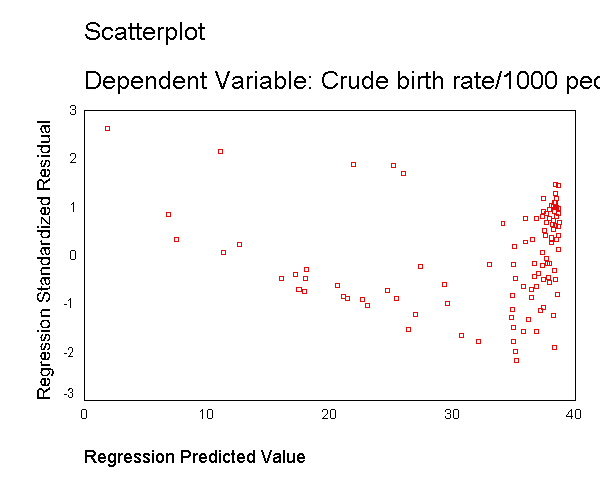Let's look at the relationship between GNP per capita (gnpcap) and births (birth).  Below if we look at the scatterplot between gnpcap and birth, we can see that the relationship between these two variables is quite non-linear. We added a regression line to the chart by double clicking on it and choosing "Chart" then "Options" and then "Fit Line Total" and you can see how poorly the line fits this data. Also, if we look at the residuals by predicted, we see that the residuals are not homoscedastic, due to the non-linearity in the relationship between gnpcap and birth.

get file = "c:sppsregnations.sav".

regression
  /dependent birth
  /method=enter gnpcap
  /scatterplot(*zresid *pred)
  /scat(birth gnpcap) .

Variables Entered/Removed(b)

Model	Variables Entered	Variables Removed	Method
1	GNPCAP(a)	.	Enter
a All requested variables entered.
b Dependent Variable: BIRTH

Model Summary(b)

Model	R	R Square	Adjusted R Square	Std. Error of the Estimate
1	.626(a)	.392	.387	10.679
a Predictors: (Constant), GNPCAP
b Dependent Variable: BIRTH

ANOVA(b)

Model		Sum of Squares	df	Mean Square	F	Sig.
1	Regression	7873.995	1	7873.995	69.047	.000(a)
	Residual	12202.152	107	114.039
	Total	20076.147	108
a Predictors: (Constant), GNPCAP
b Dependent Variable: BIRTH

Coefficients(a)

		Unstandardized Coefficients		Standardized Coefficients	t	Sig.
Model		B	Std. Error	Beta
1	(Constant)	38.924	1.261		30.856	.000
	GNPCAP	-1.921E-03	.000	-.626	-8.309	.000
a Dependent Variable: BIRTH

Residuals Statistics(a)

	Minimum	Maximum	Mean	Std. Deviation	N
Predicted Value	1.90	38.71	32.79	8.539	109
Residual	-23.18	28.10	.00	10.629	109
Std. Predicted Value	-3.618	.694	.000	1.000	109
Std. Residual	-2.170	2.632	.000	.995	109
a Dependent Variable: BIRTH

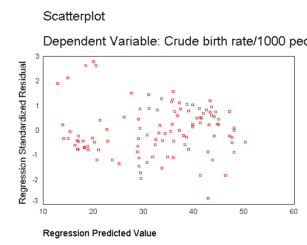
We modified the above scatterplot changing the fit line from using linear regression to using "lowess" by choosing "Chart" then "Options" then choosing "Fit Options" and choosing "Lowess" with the default smoothing parameters. As you can see, the "lowess" smoothed curve fits substantially better than the linear regression, further suggesting that the relationship between gnpcap and birth is not linear.

We can see that the capgnp scores are quite skewed with most values being near 0, and a handful of values of 10,000 and higher.  This suggests to us that some transformation of the variable may be necessary. One commonly used transformation is a log transformation, so let's try that.  As you see, the scatterplot between capgnp and birth looks much better with the regression line going through the heart of the data.  Also, the plot of the residuals by predicted values look much more reasonable.

compute lgnpcap = ln(gnpcap).
regression
  /dependent birth
  /method=enter lgnpcap
  /scatterplot(*zresid *pred) /scat(birth lgnpcap)
  /save resid(bres2).
 

Variables Entered/Removed(b)

Model	Variables Entered	Variables Removed	Method
1	LGNPCAP(a)	.	Enter
a All requested variables entered.
b Dependent Variable: BIRTH

Model Summary(b)

Model	R	R Square	Adjusted R Square	Std. Error of the Estimate
1	.756(a)	.571	.567	8.969
a Predictors: (Constant), LGNPCAP
b Dependent Variable: BIRTH

ANOVA(b)

Model		Sum of Squares	df	Mean Square	F	Sig.
1	Regression	11469.248	1	11469.248	142.584	.000(a)
	Residual	8606.899	107	80.438
	Total	20076.147	108
a Predictors: (Constant), LGNPCAP
b Dependent Variable: BIRTH

Coefficients(a)

		Unstandardized Coefficients		Standardized Coefficients	t	Sig.
Model		B	Std. Error	Beta
1	(Constant)	84.277	4.397		19.168	.000
	LGNPCAP	-7.238	.606	-.756	-11.941	.000
a Dependent Variable: BIRTH

Residuals Statistics(a)

	Minimum	Maximum	Mean	Std. Deviation	N
Predicted Value	12.86	50.25	32.79	10.305	109
Residual	-24.75	24.98	.00	8.927	109
Std. Predicted Value	-1.934	1.695	.000	1.000	109
Std. Residual	-2.760	2.786	.000	.995	109
a Dependent Variable: BIRTH

This section has shown how you can use scatterplots to diagnose problems of non-linearity, both by looking at the scatterplots of the predictor and outcome variable, as well as by examining the residuals by predicted values.  These examples have focused on simple regression, however similar techniques would be useful in multiple regression.  However, when using multiple regression, it would be more useful to examine partial regression plots instead of the simple scatterplots between the predictor variables and the outcome variable.

2.6 Model Specification

A model specification error can occur when one or more relevant variables are omitted from the model or one or more irrelevant variables are included in the model. If relevant variables are omitted from the model, the common variance they share with included variables may be wrongly attributed to those variables, and the error term can be inflated. On the other hand, if irrelevant variables are included in the model, the common variance they share with included variables may be wrongly attributed to them. Model specification errors can substantially affect the estimate of regression coefficients.

Consider the model below. This regression suggests that as class size increases the academic performance increases, with p=0.053. Before we publish results saying that increased class size is associated with higher academic performance, let's check the model specification. 

  /dependent api00
  /method=enter acs_k3 full
  /save pred(apipred).

<some output deleted to save space> 

Coefficients(a)

		Unstandardized Coefficients		Standardized Coefficients	t	Sig.
Model		B	Std. Error	Beta
1	(Constant)	32.213	84.075		.383	.702
	ACS_K3	8.356	4.303	.080	1.942	.053
	FULL	5.390	.396	.564	13.598	.000
a Dependent Variable: API00

SPSS does not have any tools that directly support the finding of specification errors, however you can check for omitted variables by using the procedure below.  As you notice above, when we ran the regression we saved the predicted value calling it apipred.  If we use the predicted value and the predicted value squared as predictors of the dependent variable, apipred should be significant since it is the predicted value, but apipred squared shouldn't be a significant predictor because, if our model is specified correctly, the squared predictions should not have much of explanatory power above and beyond the predicted value. That is we wouldn't  expect apipred squared to be a significant predictor if our model is specified correctly. Below we compute apipred2 as the squared value of apipred and then include apipred and apipred2 as predictors in our regression model, and we hope to find that apipred2 is not significant.

compute apipred2 = apipred**2.
regression
  /dependent api00
  /method=enter apipred apipred2.

<some output omitted to save space>

Coefficients(a)

		Unstandardized Coefficients		Standardized Coefficients	t	Sig.
Model		B	Std. Error	Beta
1	(Constant)	858.873	283.460		3.030	.003
	APIPRED	-1.869	.937	-1.088	-1.994	.047
	APIPRED2	2.344E-03	.001	1.674	3.070	.002
a Dependent Variable: API00

The above results show that apipred2 is significant, suggesting that we may have omitted important variables in our regression. We therefore should consider whether we should add any other variables to our model. Let's try adding the variable meals to the above model. We see that meals is a significant predictor, and we save the predicted value calling it preda for inclusion in the next analysis for testing to see whether we have any additional important omitted variables.

regression
  /dependent api00
  /method=enter acs_k3 full meals
  /save pred(preda).

<some output omitted to save space>




Coefficients(a)

		Unstandardized Coefficients		Standardized Coefficients	t	Sig.
Model		B	Std. Error	Beta
1	(Constant)	771.658	48.861		15.793	.000
	ACS_K3	-.717	2.239	-.007	-.320	.749
	FULL	1.327	.239	.139	5.556	.000
	MEALS	-3.686	.112	-.828	-32.978	.000
a Dependent Variable: API00

We now create preda2 which is the square of preda, and include both of these as predictors in our model.

compute preda2 = preda**2.
regression
  /dependent api00
  /method=enter preda preda2.

<some output omitted to save space>





Coefficients(a)

		Unstandardized Coefficients		Standardized Coefficients	t	Sig.
Model		B	Std. Error	Beta
1	(Constant)	-136.510	95.059		-1.436	.152
	PREDA	1.424	.293	1.293	4.869	.000
	PREDA2	-3.172E-04	.000	-.386	-1.455	.146
a Dependent Variable: API00

We now see that preda2 is not significant, so this test does not suggest there are any other important omitted variables.  Note that after including meals and full, the coefficient for class size is no longer significant. While acs_k3 does have a positive relationship with api00 when only full is included in the model, but when we also include (and hence control for) meals, acs_k3 is no longer significantly related to api00 and its relationship with api00 is no longer positive. 

2.7 Issues of Independence

The statement of this assumption is that the errors associated with one observation are not correlated with the errors of any other observation. Violation of this assumption can occur in a variety of situations. Consider the case of collecting data from students in eight different elementary schools. It is likely that the students within each school will tend to be more like one another that students from different schools, that is, their errors are not independent. 

Another way in which the assumption of independence can be broken is when data are collected on the same variables over time. Let's say that we collect truancy data every semester for 12 years. In this situation it is likely that the errors for observations between adjacent semesters will be more highly correlated than for observations more separated in time -- this is known as autocorrelation. When you have data that can be considered to be time-series you can use the Durbin-Watson statistic to test for correlated residuals.

We don't have any time-series data, so we will use the elemapi2 dataset and pretend that snum indicates the time at which the data were collected. We will sort the data on snum to order the data according to our fake time variable and then we can run the regression analysis with the durbin option to request the Durbin-Watson test. The Durbin-Watson statistic has a range from 0 to 4 with a midpoint of 2. The observed value in our example is less than 2, which is not surprising since our data are not truly time-series. 

sort cases by snum .
regression
  /dependent api00
  /method=enter enroll
  /residuals =  durbin .

Model Summary

Model	R	R Square	Adjusted R Square	Std. Error of the Estimate	Durbin-Watson
1	.318	.101	.099	135.026	1.351

a Predictors: (Constant), ENROLL

b Dependent Variable: API00

2.8 Summary

This chapter has covered a variety of topics in assessing the assumptions of regression using SPSS, and the consequences of violating these assumptions.  As we have seen, it is not sufficient to simply run a regression analysis, but it is important to verify that the assumptions have been met.  If this verification stage is omitted and your data does not meet the assumptions of linear regression, your results could be misleading and your interpretation of your results could be in doubt. Without  thoroughly checking your data for problems, it is possible that another researcher could analyze your data and uncover such problems and question your results showing an improved analysis that may contradict your results and undermine your conclusions. 

2.9 For more information

You can see the following web pages for more information and resources on regression diagnostics in SPSS.

• SPSS Textbook Examples- Applied Regression Analysis, Chapter 11
• SPSS Textbook Examples- Applied Regression Analysis, Chapter 12
• SPSS Textbook Examples- Applied Regression Analysis, Chapter 13
• SPSS Textbook Examples- Regression with Graphics, Chapter 4