Stata Analysis Tools Weighted Least Squares Regression

Weighted least squares provides one method for dealing with heteroscedasticity. The wls0 command can be used to compute various WLS solutions. You can download wls0 over the internet by typing search wls0 (see How can I use the search command to search for programs and get additional help? for more information about using search).

Let’s use an example dataset that exhibits heteroscedasticity, hetdata.

use https://stats.idre.ucla.edu/stat/stata/ado/analysis/hetdata, clear

regress exp age ownrent income incomesq

Source | SS df MS Number of obs = 72 -------------+------------------------------ F( 4, 67) = 5.39 Model | 1749357.01 4 437339.252 Prob > F = 0.0008 Residual | 5432562.03 67 81083.0153 R-squared = 0.2436 -------------+------------------------------ Adj R-squared = 0.1984 Total | 7181919.03 71 101153.789 Root MSE = 284.75

------------------------------------------------------------------------------ exp | Coef. Std. Err. t P>|t| [95% Conf. Interval] -------------+---------------------------------------------------------------- age | -3.081814 5.514717 -0.56 0.578 -14.08923 7.925606 ownrent | 27.94091 82.92232 0.34 0.737 -137.5727 193.4546 income | 234.347 80.36595 2.92 0.005 73.93593 394.7581 incomesq | -14.99684 7.469337 -2.01 0.049 -29.9057 -.0879859 _cons | -237.1465 199.3517 -1.19 0.238 -635.0541 160.7611 ------------------------------------------------------------------------------

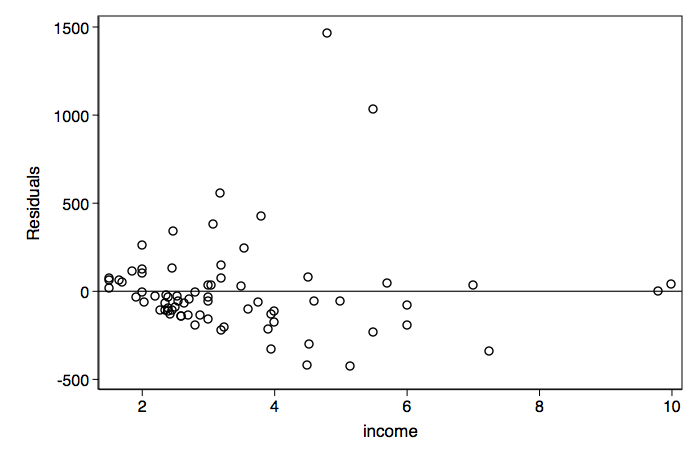
rvpplot income, yline(0) scheme(lean1)

Image het1

The residual versus income plot shows clear evidence of heteroscedasticity. Let's try a WLS weighting proportional to income. The WLS type, abse, uses the absolute value of the residuals and in this case no constant.

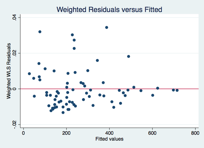
wls0 exp age ownrent income incomesq, wvar(income) type(abse) noconst graph

WLS regression - type: proportional to abs(e)

(sum of wgt is 5.1961e-03)

Source | SS df MS Number of obs = 72 -------------+------------------------------ F( 4, 67) = 5.73 Model | 818838.784 4 204709.696 Prob > F = 0.0005 Residual | 2393372.07 67 35721.9713 R-squared = 0.2549 -------------+------------------------------ Adj R-squared = 0.2104 Total | 3212210.86 71 45242.4065 Root MSE = 189

------------------------------------------------------------------------------ exp | Coef. Std. Err. t P>|t| [95% Conf. Interval] -------------+---------------------------------------------------------------- age | -2.694186 3.807306 -0.71 0.482 -10.2936 4.905229 ownrent | 60.44878 58.55088 1.03 0.306 -56.41928 177.3168 income | 158.427 76.39115 2.07 0.042 5.949594 310.9044 incomesq | -7.249289 9.724337 -0.75 0.459 -26.65915 12.16057 _cons | -114.1089 139.6875 -0.82 0.417 -392.9263 164.7085 ------------------------------------------------------------------------------

Image het2

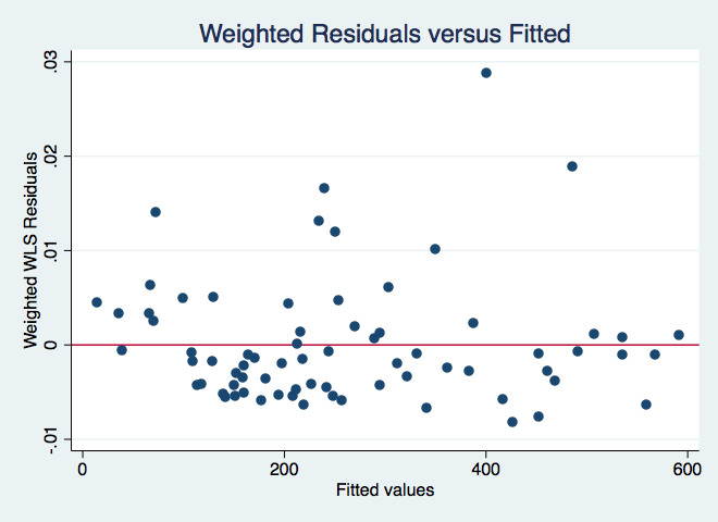
The residual plot is better. We can try other possibilities, such as, weighting proportional to income and income squared.

wls0 exp age ownrent income incomesq, wvar(income incomesq) type(abse) noconst graph

WLS regression - type: proportional to abs(e)

(sum of wgt is 2.7071e-03)

Source | SS df MS Number of obs = 72 -------------+------------------------------ F( 4, 67) = 7.60 Model | 1481099.44 4 370274.86 Prob > F = 0.0000 Residual | 3265263.26 67 48735.2725 R-squared = 0.3120 -------------+------------------------------ Adj R-squared = 0.2710 Total | 4746362.7 71 66850.1788 Root MSE = 220.76

------------------------------------------------------------------------------ exp | Coef. Std. Err. t P>|t| [95% Conf. Interval] -------------+---------------------------------------------------------------- age | -2.927867 4.412377 -0.66 0.509 -11.73501 5.879275 ownrent | 51.12242 67.95408 0.75 0.455 -84.51449 186.7593 income | 196.4813 62.26251 3.16 0.002 72.20479 320.7578 incomesq | -11.95962 5.511042 -2.17 0.034 -22.95971 -.9595377 _cons | -166.6852 145.0887 -1.15 0.255 -456.2834 122.913 ------------------------------------------------------------------------------

Image het3

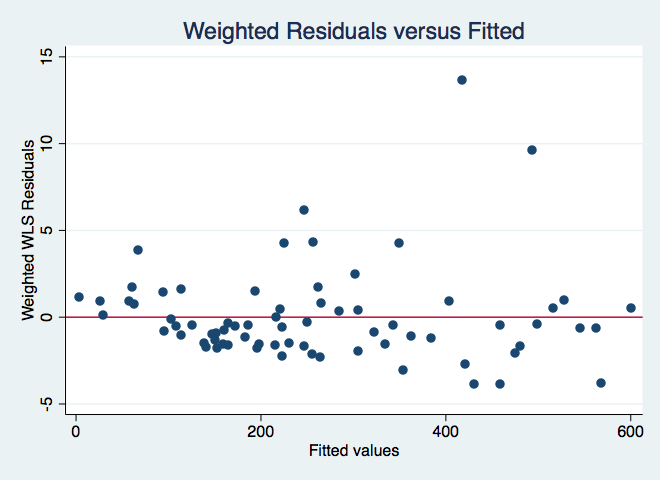
Finally, let's try one more variation. This time we will make the adjustment proportional to the log of squared residuals.

wls0 exp age ownrent income incomesq, wvar(income incomesq) type(loge2) graph

WLS regression - type: proportional to log(e)^2

(sum of wgt is 9.3775e-01)

Source | SS df MS Number of obs = 72 -------------+------------------------------ F( 4, 67) = 7.93 Model | 1953755.81 4 488438.951 Prob > F = 0.0000 Residual | 4126765.99 67 61593.5222 R-squared = 0.3213 -------------+------------------------------ Adj R-squared = 0.2808 Total | 6080521.79 71 85641.152 Root MSE = 248.18

------------------------------------------------------------------------------ exp | Coef. Std. Err. t P>|t| [95% Conf. Interval] -------------+---------------------------------------------------------------- age | -3.020919 4.93586 -0.61 0.543 -12.87294 6.831099 ownrent | 40.31746 76.15911 0.53 0.598 -111.6968 192.3317 income | 213.373 66.55042 3.21 0.002 80.53779 346.2082 incomesq | -13.27511 5.514378 -2.41 0.019 -24.28185 -2.268364 _cons | -197.3543 168.7816 -1.17 0.246 -534.2439 139.5353 ------------------------------------------------------------------------------

Image het4

In addition to weight types abse and loge2 there is squared residuals (e2) and squared fitted values (xb2).

Finding the optimal WLS solution to use involves detailed knowledge of your data and trying different combinations of variables and types of weighting.