Purpose: The regpt command is a teaching tool for showing the influence of one point in a regression analysis, allowing you to see how the point influences the regression line, using OLS regression, Robust regression, or Quantile Regression. It also allows you to see how such problems are revealed using some common regression diagnostic graphs.
Download: You can download this program from within Stata by typing search regpt (see How can I used the search command to search for programs and get additional help? for more information about using search).
Use of program: To use this program, type regpt in the Stata command window. When you start regpt with no options it generates 30 observations drawn from a population with a correlation of .30 and displays the scatterplot of the data with the regression line. You can use the n( ) option to specify a different sample size and the r( ) option to specify a different correlation. After the program starts, a scatterplot with the regression line is shown, and a dialog box is opened allowing you to move a single point to see how it affects the regression line. The y+.5 and y-.5 buttons allow you to move the point in the y axis, and the x+.5 and x-.5 buttons allow you to shift the moving point in the X axis (while keeping the distance from the regression line on the y axis constant).
By default, a scatterplot with OLS regression line is shown, but you can use the Choose Plot Type pulldown to select other plots, including a scatterplot with robust regression line, a scatterplot with a quantile regression line, a residual vs. fitted plot, leverage vs. residual squared, and a leverage vs. residual squared with Cook’s D.
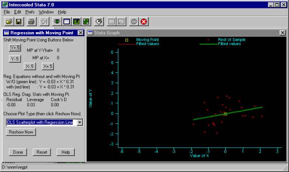
Examples: Below we start regpt with no options and it generates 30 observations drawn from a population where the correlation between X and Y is .30 and displays the scatterplot of the data with the regression line. In Figure 1, you see the scatterplot it created (at the right) and a dialog box at the left. The dialog box allows you to shift the moving point (shown as a yellow square) that is initially positioned on the regression line and at X=0, as shown below. We can move this point and see how moving this single point influences the regression line.
Figure
1. Regpt output with X=0 and Y-Yhat=0
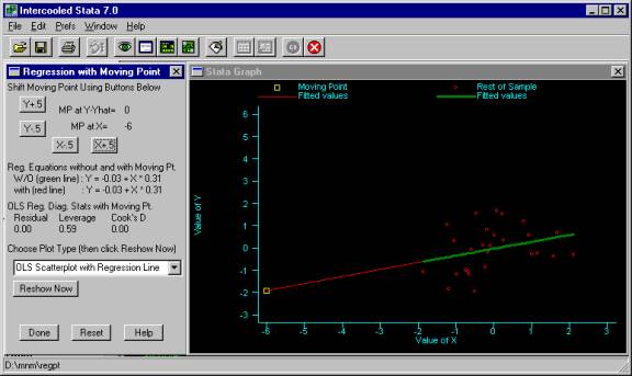
If we decrease the value of X (by pressing the X-.5 button), the point moves along the regression line. We see no difference between the regression line with the moving point (the thin line), and the regression line without the moving point (the thick line). We can confirm this by looking at the regression equation without and with the moving point and see that the formula for the regression is the same whether we include the moving point or not. Looking at the OLS Reg. Diag. Stats with Moving Pt. we see that when we moved the values of X, the residual and Cook s D did not change, but the leverage increased, see Figure 2. (Note that as you change the values of X, the residual remains unchanged. This allows you to see the effect of changing X while keeping the residual constant. )
Figure
2. Regpt output with X= -6 and Y-Yhat= 0
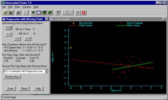
We can change the value of Y by pressing the Y+.5 button. As we increase the value of Y we see that the point causes a great discrepancy between the regression line with the moving point (the thin line) and the regression line without the moving point (the thick line), see Figure 3. The dialog at the left shows us the numeric impact on the coefficient for the slope; without the moving point, the slope is .31, but with the moving point the coefficient is -.17. Looking at the diagnostic statistics, we can see the leverage did not change as we changed the value of Y, but the residual and Cook s D changed quite a bit. The large value for Cook s D reflects the strong impact this one point has on the regression results.
Figure
3. Regpt output with X= -6 and Y-Yhat= 5
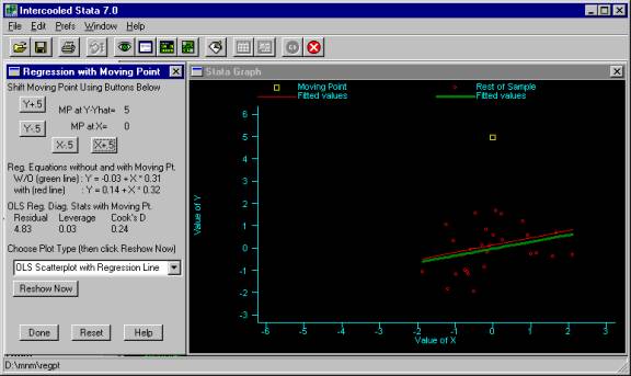
We can then shift the value of X for the moving point back to 0 by pressing X+.5 and we see that the influence of the moving point on the slope of the line diminishes, see Figure 4. (Again, please note that when we change X, the value of Y changes, but the residual remains constant. This allows us to see the effect of changing X while holding the residual constant.) With X returned to 0, the moving point has no real effect on the slope of the regression line. The only real effect of this point is to lift the regression line, increasing the intercept. Looking at the regression diagnostics for this point, we see its leverage is virtually 0, but has a high residual (since it is far from the regression line). Although this point has a high residual, the Cook s D for this point is not very large (.24) because it does not exert a large influence on the slope of the line.
Figure
4. Regpt output with X= 0 and Y-Yhat= 5
In addition to showing a scatterplot with a regression line, you can choose a variety of other plots using Choose Plot Type . For example, we can select Leverage vs. Residual Squared plot and then click Reshow Now to show the plot, see Figure 5. This shows us that the moving point has a very large residual (as compared to the other points) but has very low leverage. This corresponds to what we saw in Figure 4, where the moving point was very different from the rest of the points but did not exert much influence on the regression results.
Figure
5. Regpt Leverage vs. Residual output with X= -6 and Y-Yhat= 0
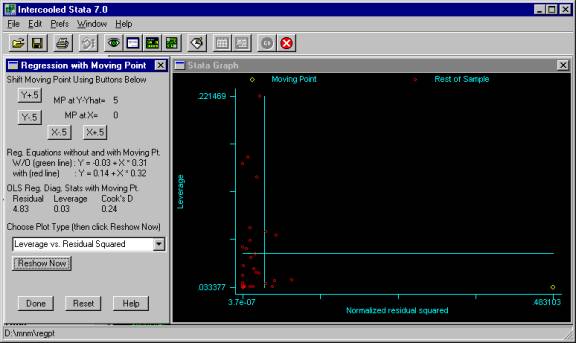
There are other plot types we could choose. We could choose to show the plot using Robust Regression, which allows you to see the influence of a single point in robust regression. If you repeat the steps shown above with robust regression, you would see that as the moving point gets more and more outlying, its influence is attenuated until the weighting of the point goes to 0 and it is effectively eliminated. Likewise, we could show the plot using quantile regression, and again it would show the diminishing influence of an influential single point. Other options for the Show Plot As include showing a Residual vs. Fitted plot , a Leverage vs. Residual Squared plot (shown in Figure 5), and a Leverage vs. Residual Squared Plot with the size of the symbols weighted by Cook s D.
Summary. We created this tool to be able to better understand how a single outlier influences the regression line and how regression diagnostic tools reveal underlying problems. It seems apt that we use the term regression diagnostics , because we are trying to diagnose various kinds of illnesses in our data based on symptoms (like leverage or Cook s D or residual vs. fitted plots). Using regpt you can cause a particular kind of problem (illness), and then see the symptoms it manifests in the numeric diagnostic tools we use (e.g. the residual, leverage, and Cook s D) and graphical diagnostic tools (e.g. residual vs. fitted plots, and leverage vs. residual squared plots). By being able to create problems and then diagnose them, we hope that regpt can help students and researchers improve their skills in inferring problems given the symptoms shown in real world regression analyses.
