Using postgr3 with multiple regression, no interactions
Using postgr3 with multiple regression, with interactions
More on options when using postgr3
postgr3 with other estimation models
This page will illustrate the use of postgr3
for making graphs after estimation commands. You can obtain postgr3 over the
internet by typing search postgr3 (see
How can I use the search command to search for programs and get additional
help? for more information about using search).
NOTE! You must install the
spostado utilities before postgr3 will work
properly. You can download spostado by typing search spostado
We also recommend obtaining the latest version of xi3 which compliments postgr3. You can download xi3 from within Stata by typing search xi3 (see How can I use the search command to search for programs and get additional help? for more information about using search). For postgr3 to work properly you need Stata 8 and your Stata should be up to date (i.e., you need to have recently run the update all command in Stata).
In these examples, we will use the hsb2 data file which you can get like this.
use https://stats.idre.ucla.edu/stat/stata/notes/hsb2, clear
Using postgr3 with multiple regression, no interactions
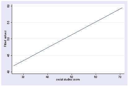
We can do a multiple regression and then show how the predicted values vary as a function of socst holding other variables constant at their mean. Note how we precede the regress command with xi3. This is because xi3 and postgr3 work together as a team.
xi3: regress read female ses socst science

      Source |       SS       df       MS              Number of obs =     200
-------------+------------------------------           F(  4,   195) =   56.33
       Model |  11214.2588     4   2803.5647           Prob > F      =  0.0000
    Residual |  9705.16119   195  49.7700574           R-squared     =  0.5361
-------------+------------------------------           Adj R-squared =  0.5266
       Total |    20919.42   199  105.122714           Root MSE      =  7.0548

------------------------------------------------------------------------------
        read |      Coef.   Std. Err.      t    P>|t|     [95% Conf. Interval]
-------------+----------------------------------------------------------------
      female |  -.3283535   1.026784    -0.32   0.749     -2.35338    1.696673
         ses |   .4767216   .7469296     0.64   0.524    -.9963759    1.949819
       socst |   .3941527    .054806     7.19   0.000     .2860642    .5022413
     science |   .4418034   .0584274     7.56   0.000     .3265726    .5570343
       _cons |   7.866209   3.125707     2.52   0.013     1.701677    14.03074
------------------------------------------------------------------------------

postgr3 socst

Variables left asis: socst
Holding female constant at .545
Holding ses constant at 2.055
Holding science constant at 51.85
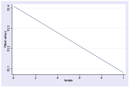
We can show how the predicted values vary as a function of female holding other variables constant at their mean.
postgr3 female

Variables left asis: female
Holding ses constant at 2.055
Holding socst constant at 52.405
Holding science constant at 51.85
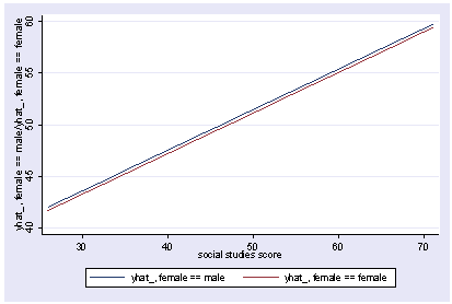
We can also show how the predicted values vary as a function of socst and female, holding other variables constant at their mean.
postgr3 socst, by(female)

Variables left asis: socst female
Holding ses constant at 2.055
Holding science constant at 51.85
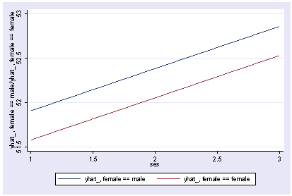
Or we can show how the predicted values vary by ses and female, holding other variables constant at their mean.
postgr3 ses, by(female)

Variables left asis: ses female
Holding socst constant at 52.405
Holding science constant at 51.85
Using postgr3 with multiple regression, with interactions
If we wish to include categorical variables (especially interactions), we then use xi3 for coding the categorical variables. Although it permits a wide variety of coding schemes (see help xi3) we will just use regular dummy coding indicated by the i. prefix. We wull run the above model with an interaction of socst and female and show the graph of the interaction, holding other variables constant at their mean.
xi3: regress read i.female*socst ses science

i.female          _Ifemale_0-1        (naturally coded; _Ifemale_0 omitted)
i.female*socst    _IfemXsocst_#       (coded as above)

      Source |       SS       df       MS              Number of obs =     200
-------------+------------------------------           F(  5,   194) =   45.29
       Model |  11267.2025     5   2253.4405           Prob > F      =  0.0000
    Residual |   9652.2175   194  49.7536985           R-squared     =  0.5386
-------------+------------------------------           Adj R-squared =  0.5267
       Total |    20919.42   199  105.122714           Root MSE      =  7.0536

------------------------------------------------------------------------------
        read |      Coef.   Std. Err.      t    P>|t|     [95% Conf. Interval]
-------------+----------------------------------------------------------------
  _Ifemale_1 |  -5.363727   4.988108    -1.08   0.284    -15.20161    4.474156
       socst |   .3453355   .0724033     4.77   0.000     .2025369    .4881342
_IfemXsocs~1 |    .096356   .0934081     1.03   0.304    -.0878697    .2805817
         ses |   .5139953   .7476804     0.69   0.493    -.9606305    1.988621
     science |   .4425136   .0584219     7.57   0.000       .32729    .5577372
       _cons |   10.27643   3.902047     2.63   0.009     2.580547    17.97231
------------------------------------------------------------------------------

postgr3 socst, by(female)

Variables left asis: socst _Ifemale_1 _IfemXsocst_1
Holding ses constant at 2.055
Holding science constant at 51.85
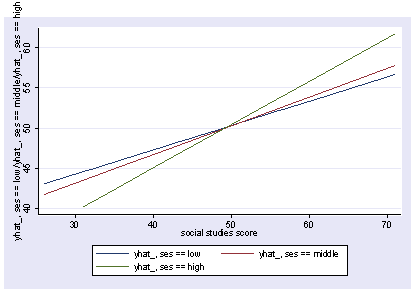
We can use reverse helmert coding on ses (which compares 2 vs 1 and 3 vs 12) and interact that by socst and then use postgr3 to show this interaction, holding other variables constant.
xi3: regress read r.ses*socst female science

r.ses             _Ises_1-3           (naturally coded; _Ises_1 omitted)
r.ses*socst       _IsesXsocst_#       (coded as above)

      Source |       SS       df       MS              Number of obs =     200
-------------+------------------------------           F(  7,   192) =   32.99
       Model |  11421.7692     7  1631.68131           Prob > F      =  0.0000
    Residual |  9497.65083   192  49.4669314           R-squared     =  0.5460
-------------+------------------------------           Adj R-squared =  0.5294
       Total |    20919.42   199  105.122714           Root MSE      =  7.0333

------------------------------------------------------------------------------
        read |      Coef.   Std. Err.      t    P>|t|     [95% Conf. Interval]
-------------+----------------------------------------------------------------
     _Ises_2 |  -2.790321   6.033969    -0.46   0.644     -14.6917    9.111058
     _Ises_3 |   -10.3084   6.228643    -1.65   0.100    -22.59375    1.976956
       socst |   .4011395   .0560911     7.15   0.000     .2905057    .5117734
_IsesXsocs~2 |   .0552476   .1203009     0.46   0.647    -.1820334    .2925285
_IsesXsocs~3 |   .2089692   .1119203     1.87   0.063     -.011782    .4297204
      female |   -.196438   1.033133    -0.19   0.849    -2.234185    1.841309
     science |   .4375687   .0582931     7.51   0.000     .3225916    .5525459
       _cons |   8.327722   3.304713     2.52   0.013     1.809518    14.84593
------------------------------------------------------------------------------

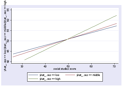
postgr3 socst, by(ses)

Variables left asis: socst _Ises_2 _Ises_3 _IsesXsocst_2 _IsesXsocst_3
Holding female constant at .545
Holding science constant at 51.85
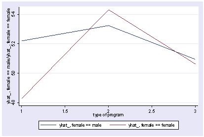
We can use reverse helmert coding on prog and look at the interaction with female using xi3 and then show the interaction with postgr3.
xi3: regress read r.prog*i.female socst  science

r.prog            _Iprog_1-3          (naturally coded; _Iprog_1 omitted)
i.female          _Ifemale_0-1        (naturally coded; _Ifemale_0 omitted)
r.prog*i.female   _IproXfem_#_#       (coded as above)

      Source |       SS       df       MS              Number of obs =     200
-------------+------------------------------           F(  7,   192) =   36.05
       Model |  11879.6717     7  1697.09595           Prob > F      =  0.0000
    Residual |  9039.74835   192  47.0820227           R-squared     =  0.5679
-------------+------------------------------           Adj R-squared =  0.5521
       Total |    20919.42   199  105.122714           Root MSE      =  6.8616

------------------------------------------------------------------------------
        read |      Coef.   Std. Err.      t    P>|t|     [95% Conf. Interval]
-------------+----------------------------------------------------------------
    _Iprog_2 |   1.044267   1.826394     0.57   0.568    -2.558106     4.64664
    _Iprog_3 |   -1.78684    1.78787    -1.00   0.319    -5.313229    1.739548
  _Ifemale_1 |  -1.053392   1.058655    -1.00   0.321    -3.141479    1.034694
_IproXfe~2_1 |   5.005482    2.45381     2.04   0.043     .1655968    9.845368
_IproXfe~3_1 |   1.114799   2.312977     0.48   0.630    -3.447309    5.676906
       socst |    .339437   .0561575     6.04   0.000     .2286722    .4502018
     science |   .4448466   .0568237     7.83   0.000     .3327678    .5569255
       _cons |   11.27162   3.240477     3.48   0.001     4.880115    17.66313
------------------------------------------------------------------------------

postgr3 prog, by(female)

Variables left asis: _Iprog_2 _Iprog_3 _Ifemale_1 _IproXfem_2_1 _IproXfem_3_1
Holding socst constant at 52.405
Holding science constant at 51.85
More on options when using postgr3
Let us consider this regression model with an interaction term for ses and socst.
xi3: regress read r.ses*socst female science

r.ses             _Ises_1-3           (naturally coded; _Ises_1 omitted)
r.ses*socst       _IsesXsocst_#       (coded as above)

      Source |       SS       df       MS              Number of obs =     200
-------------+------------------------------           F(  7,   192) =   32.99
       Model |  11421.7692     7  1631.68131           Prob > F      =  0.0000
    Residual |  9497.65083   192  49.4669314           R-squared     =  0.5460
-------------+------------------------------           Adj R-squared =  0.5294
       Total |    20919.42   199  105.122714           Root MSE      =  7.0333

------------------------------------------------------------------------------
        read |      Coef.   Std. Err.      t    P>|t|     [95% Conf. Interval]
-------------+----------------------------------------------------------------
     _Ises_2 |  -2.790321   6.033969    -0.46   0.644     -14.6917    9.111058
     _Ises_3 |   -10.3084   6.228643    -1.65   0.100    -22.59375    1.976956
       socst |   .4011395   .0560911     7.15   0.000     .2905057    .5117734
_IsesXsocs~2 |   .0552476   .1203009     0.46   0.647    -.1820334    .2925285
_IsesXsocs~3 |   .2089692   .1119203     1.87   0.063     -.011782    .4297204
      female |   -.196438   1.033133    -0.19   0.849    -2.234185    1.841309
     science |   .4375687   .0582931     7.51   0.000     .3225916    .5525459
       _cons |   8.327722   3.304713     2.52   0.013     1.809518    14.84593
------------------------------------------------------------------------------
As we have seen, we can show the interaction with postgr3 like below.
postgr3 socst, by(ses)

Variables left asis: socst _Ises_2 _Ises_3 _IsesXsocst_2 _IsesXsocst_3
Holding female constant at .545
Holding science constant at 51.85
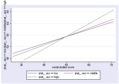
We can use the x option to show the predicted values with other variables held constant at different values than the mean. For example, we can show the predicted values for females with science scores of 60.
postgr3 socst, by(ses) x(female=1 science=60)

Variables left asis: socst _Ises_2 _Ises_3 _IsesXsocst_2 _IsesXsocst_3
Holding female constant at 1
Holding science constant at 60
If we use the x option to show the predicted values for females and make no reference to science, then science will be held at the overall mean of science (for males and females). Instead, we can use rest(grmean) to indicate that the rest of the variables should be held at the group mean as indicated by the x variable. So, if we did summarize if female==1 and got that mean for science it would be 50.69. As you see below, science is held constant at that value, the mean for females.
postgr3 socst, by(ses) x(female=1) rest(grmean)

Variables left asis: socst _Ises_2 _Ises_3 _IsesXsocst_2 _IsesXsocst_3
Holding female constant at 1
Holding science constant at 50.697248
We can show a table of the predicted values using the table option, as shown below. Note that missing values are indicated where no observations were present (the graph is omitted to save space).
postgr3 socst, by(ses) x(female=1) rest(grmean) table

Variables left asis: socst _Ises_2 _Ises_3 _IsesXsocst_2 _IsesXsocst_3
Holding female constant at 1
Holding science constant at 50.697248
predict yhat_,
(option xb assumed; fitted values)

                          Means of Fitted values

    social |
   studies |              ses
     score |       low     middle       high |     Total
-----------+---------------------------------+----------
        26 | 43.046452  41.692566          . | 42.595156
        31 | 44.565746  43.488102  40.196571 |  42.93463
        32 | 44.869606          .          . | 44.869606
        33 | 45.173466          .          . | 45.173466
        36 | 46.085045  45.283634  42.898834 | 45.286063
        37 | 46.388905          .          . | 46.388905
        39 |         .          .  44.520191 | 44.520191
        41 |  47.60434   47.07917  45.601097 | 47.117067
        42 |         .          .  46.141548 | 46.141548
        43 | 48.212059          .          . | 48.212059
        44 | 48.515919          .          . | 48.515919
        46 | 49.123638  48.874702   48.30336 | 48.825146
        47 |         .          .  48.843811 | 48.843811
        48 | 49.731358          .          . | 49.731358
        51 | 50.642933  50.670238  51.005619 | 50.695648
        52 |         .  51.029346  51.546074 |  51.28771
        56 | 52.162231  52.465775  53.707882 | 52.787533
        57 | 52.466091          .          . | 52.466091
        58 |         .  53.183987          . | 53.183987
        61 | 53.681526  54.261307  56.410145 | 55.202913
        66 | 55.200825  56.056843  59.112404 | 57.604936
        71 | 56.720119  57.852375  61.814667 | 59.691989
-----------+---------------------------------+----------
     Total | 49.524473  51.040686  54.322879 | 51.636212
If we show the predicted values by 2 categorical variables, we might also want to show a table of the predicted values, for example broken down by prog and female as illustrated below.
xi3: regress read r.prog*i.female socst  science

r.prog            _Iprog_1-3          (naturally coded; _Iprog_1 omitted)
i.female          _Ifemale_0-1        (naturally coded; _Ifemale_0 omitted)
r.prog*i.female   _IproXfem_#_#       (coded as above)

      Source |       SS       df       MS              Number of obs =     200
-------------+------------------------------           F(  7,   192) =   36.05
       Model |  11879.6717     7  1697.09595           Prob > F      =  0.0000
    Residual |  9039.74835   192  47.0820227           R-squared     =  0.5679
-------------+------------------------------           Adj R-squared =  0.5521
       Total |    20919.42   199  105.122714           Root MSE      =  6.8616

------------------------------------------------------------------------------
        read |      Coef.   Std. Err.      t    P>|t|     [95% Conf. Interval]
-------------+----------------------------------------------------------------
    _Iprog_2 |   1.044267   1.826394     0.57   0.568    -2.558106     4.64664
    _Iprog_3 |   -1.78684    1.78787    -1.00   0.319    -5.313229    1.739548
  _Ifemale_1 |  -1.053392   1.058655    -1.00   0.321    -3.141479    1.034694
   _Ipr2Xfe1 |   5.005482    2.45381     2.04   0.043     .1655968    9.845368
   _Ipr3Xfe1 |   1.114799   2.312977     0.48   0.630    -3.447309    5.676906
       socst |    .339437   .0561575     6.04   0.000     .2286722    .4502018
     science |   .4448466   .0568237     7.83   0.000     .3327678    .5569255
       _cons |   11.27162   3.240477     3.48   0.001     4.880115    17.66313
------------------------------------------------------------------------------

postgr3 prog, by(female) table

Variables left asis: _Iprog_2 _Iprog_3 _Ifemale_1 _IproXfem_2_1 _IproXfem_3_1
Holding socst constant at 52.405
Holding science constant at 51.85
                          Means of Fitted values

   type of |       female
   program |      male     female |     Total
-----------+----------------------+----------
   general | 52.198593  48.270859 | 50.103801
  academic | 53.242859   54.32061 | 53.838188
  vocation | 50.933884  50.623692 |  50.76638
-----------+----------------------+----------
     Total | 52.418287  52.072804 | 52.229999
However, the table is not in the same orientation as the graph, so you can use the table2 option to swap the rows and columns of the table and to make it better correspond with the graph.
postgr3 prog, by(female) table2

Variables left asis: _Iprog_2 _Iprog_3 _Ifemale_1 _IproXfem_2_1 _IproXfem_3_1
Holding socst constant at 52.405
Holding science constant at 51.85
                          Means of Fitted values

           |        type of program
    female |   general   academic   vocation |     Total
-----------+---------------------------------+----------
      male | 52.198593  53.242859  50.933884 | 52.418287
    female | 48.270859   54.32061  50.623692 | 52.072804
-----------+---------------------------------+----------
     Total | 50.103801  53.838188   50.76638 | 52.229999
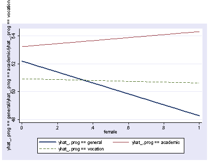
We can add graph options to make the graph look better. For example, below we add the clpattern() and the clwidth() options to control the line pattern and line width.
postgr3 female, by(prog) clpattern(l l dash ) clwidth(thick . .)

Variables left asis: _Ifemale_1 _Iprog_2 _Iprog_3 _Ipr2Xfe1 _Ipr3Xfe1
Holding socst constant at 52.405
Holding science constant at 51.85
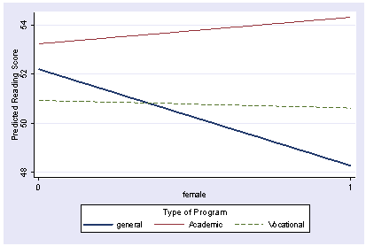
We can add additional graph options to make the graph look nicer. We add lagend options, and change the ytitle and labels for the x axis below to improve the look of the graph.
postgr3 female, by(prog) clpattern(l l dash ) clwidth(thick . .) ///
    legend(subtitle(Type of Program) order(1 "general" 2 "Academic" 3 "Vocational") rows(1) ) ///
    ytitle(Predicted Reading Score) xlabel(0 1)

Variables left asis: _Ifemale_1 _Iprog_2 _Iprog_3 _Ipr2Xfe1 _Ipr3Xfe1
Holding socst constant at 52.405
Holding science constant at 51.85
Say we want to include a squared term, say socst and socst2.
gen socst2 = socst*socst
xi3: regress read r.prog*i.female socst socst2 science

r.prog            _Iprog_1-3          (naturally coded; _Iprog_1 omitted)
i.female          _Ifemale_0-1        (naturally coded; _Ifemale_0 omitted)
r.prog*i.female   _IproXfem_#_#       (coded as above)

      Source |       SS       df       MS              Number of obs =     200
-------------+------------------------------           F(  8,   191) =   32.48
       Model |  12057.4759     8  1507.18449           Prob > F      =  0.0000
    Residual |   8861.9441   191  46.3976131           R-squared     =  0.5764
-------------+------------------------------           Adj R-squared =  0.5586
       Total |    20919.42   199  105.122714           Root MSE      =  6.8116

------------------------------------------------------------------------------
        read |      Coef.   Std. Err.      t    P>|t|     [95% Conf. Interval]
-------------+----------------------------------------------------------------
    _Iprog_2 |   .8859053   1.814874     0.49   0.626    -2.693866    4.465676
    _Iprog_3 |  -2.339243    1.79712    -1.30   0.195    -5.883994    1.205508
  _Ifemale_1 |  -.9018447   1.053779    -0.86   0.393    -2.980384    1.176695
   _Ipr2Xfe1 |    4.74971   2.439411     1.95   0.053     -.061935    9.561356
   _Ipr3Xfe1 |   1.508573   2.304899     0.65   0.514    -3.037751    6.054898
       socst |  -.4043657   .3840249    -1.05   0.294     -1.16184    .3531089
      socst2 |   .0074461   .0038037     1.96   0.052    -.0000565    .0149488
     science |   .4234667   .0574567     7.37   0.000     .3101355    .5367979
       _cons |   29.99129   10.08915     2.97   0.003     10.09083    49.89176
------------------------------------------------------------------------------
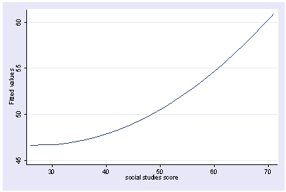
If we want to view the results as a function of socst, we would not want socst2 to be held constant. In fact, we would want that to vary as is, so we would include socst and socst2 in the asis option to prevent postgr3 from trying to hold them constant.
postgr3 socst, asis(socst socst2)

Variables left asis: socst socst2
Holding _Iprog_2 constant at .15
Holding _Iprog_3 constant at -.08333333
Holding _Ifemale_1 constant at .545
Holding _IproXfem_2_1 constant at .085
Holding _IproXfem_3_1 constant at -.04666667
Holding science constant at 51.85
postgr3 with other estimation models
Although all of the examples up to now have used regression models via the regress command, postgr3 can be used with a wide variety of estimation commands, including logit, probit, ologit, mlogit, and more. Here are some examples.
We will create a variable called goodread which is 1 if the reading score is over 60.
gen goodread = read > 60
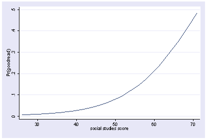
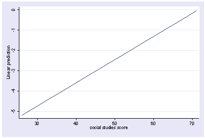
We can then use logit with and show the predicted values by socst. The y axis is showing predicted probabilities.
xi3: logit goodread i.female socst science

i.female          _Ifemale_0-1        (naturally coded; _Ifemale_0 omitted)

Iteration 0:   log likelihood = -109.04953
Iteration 1:   log likelihood = -75.950592
Iteration 2:   log likelihood = -69.751911
Iteration 3:   log likelihood =  -68.82564
Iteration 4:   log likelihood = -68.792504
Iteration 5:   log likelihood = -68.792448

Logit estimates                                   Number of obs   =        200
                                                  LR chi2(3)      =      80.51
                                                  Prob > chi2     =     0.0000
Log likelihood = -68.792448                       Pseudo R2       =     0.3692

------------------------------------------------------------------------------
    goodread |      Coef.   Std. Err.      z    P>|z|     [95% Conf. Interval]
-------------+----------------------------------------------------------------
  _Ifemale_1 |  -.0075975   .4446729    -0.02   0.986    -.8791404    .8639453
       socst |   .1140219    .027665     4.12   0.000     .0597994    .1682443
     science |   .1479431   .0340121     4.35   0.000     .0812806    .2146056
       _cons |  -15.81825   2.477648    -6.38   0.000    -20.67435   -10.96215
------------------------------------------------------------------------------

postgr3  socst

Variables left asis: socst
Holding _Ifemale_1 constant at .545
Holding science constant at 51.85
If we wished, we could show the predicted values as logits by specifying the predict option. The predict option accepts the same values as would follow the comma after the predict command.
postgr3  socst, predict(xb)

Variables left asis: socst
Holding _Ifemale_1 constant at .545
Holding science constant at 51.85
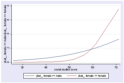
We can include an interaction of female and socst and show the predicted values holding science constant at its mean.
xi3: logit goodread i.female*socst science

i.female          _Ifemale_0-1        (naturally coded; _Ifemale_0 omitted)
i.female*socst    _IfemXsocst_#       (coded as above)

Iteration 0:   log likelihood = -109.04953
Iteration 1:   log likelihood = -75.075084
Iteration 2:   log likelihood = -67.681437
Iteration 3:   log likelihood =  -65.89615
Iteration 4:   log likelihood = -65.703276
Iteration 5:   log likelihood = -65.700115
Iteration 6:   log likelihood = -65.700114

Logit estimates                                   Number of obs   =        200
                                                  LR chi2(4)      =      86.70
                                                  Prob > chi2     =     0.0000
Log likelihood = -65.700114                       Pseudo R2       =     0.3975

------------------------------------------------------------------------------
    goodread |      Coef.   Std. Err.      z    P>|z|     [95% Conf. Interval]
-------------+----------------------------------------------------------------
  _Ifemale_1 |  -9.307788    4.19752    -2.22   0.027    -17.53478     -1.0808
       socst |   .0662987   .0307774     2.15   0.031     .0059761    .1266214
     _IfeXso |   .1571849   .0698483     2.25   0.024     .0202846    .2940851
     science |   .1479992   .0339313     4.36   0.000      .081495    .2145033
       _cons |  -13.10211   2.579092    -5.08   0.000    -18.15704   -8.047181
------------------------------------------------------------------------------

postgr3 socst, by(female)

Variables left asis: socst _Ifemale_1 _IfemXsocst_1
Holding science constant at 51.85
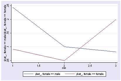
We can include an interaction of 2 categorical variables and show the predicted probabilities along with a table.
xi3: logit goodread i.ses*i.female socst science

i.ses             _Ises_1-3           (naturally coded; _Ises_1 omitted)
i.female          _Ifemale_0-1        (naturally coded; _Ifemale_0 omitted)
i.ses*i.female    _IsesXfem_#_#       (coded as above)

Iteration 0:   log likelihood = -109.04953
Iteration 1:   log likelihood = -72.980799
Iteration 2:   log likelihood = -66.566231
Iteration 3:   log likelihood = -65.555596
Iteration 4:   log likelihood = -65.512747
Iteration 5:   log likelihood = -65.512645

Logit estimates                                   Number of obs   =        200
                                                  LR chi2(7)      =      87.07
                                                  Prob > chi2     =     0.0000
Log likelihood = -65.512645                       Pseudo R2       =     0.3992

------------------------------------------------------------------------------
    goodread |      Coef.   Std. Err.      z    P>|z|     [95% Conf. Interval]
-------------+----------------------------------------------------------------
     _Ises_2 |  -1.062254   .9440273    -1.13   0.260    -2.912514    .7880054
     _Ises_3 |  -1.289494   1.022621    -1.26   0.207    -3.293795    .7148073
  _Ifemale_1 |  -1.164263   1.074516    -1.08   0.279    -3.270276    .9417497
   _Ise2Xfe1 |   .4015754   1.245133     0.32   0.747    -2.038841    2.841992
   _Ise2Xfe1 |   2.195925   1.305186     1.68   0.092    -.3621935    4.754043
       socst |   .1279548   .0310952     4.11   0.000     .0670093    .1889003
     science |   .1330011   .0345899     3.85   0.000     .0652062    .2007959
       _cons |  -14.73353   2.553764    -5.77   0.000    -19.73881   -9.728241
------------------------------------------------------------------------------

postgr3 ses, by(female) table2

Variables left asis: _Ises_2 _Ises_3 _Ifemale_1 _IsesXfem_2_1 _IsesXfem_3_1
Holding socst constant at 52.405
Holding science constant at 51.85
---------------------------------------- | ses female | low middle high ----------+----------------------------- male | .243801 .100272 .0815519 female | .0914369 .0494117 .1994422 ----------------------------------------
We can create a 3 level variable for read called readcat that will be 1 if less than 40, 2 if between 40 and 60, and 3 if over 60. We can then use ologit to predict this 3 level variable.
generate readcat = read
recode readcat 0/40=1 60/100=3 40/60=2
We then run ologit as shown below.
xi3: ologit readcat i.female*socst science

i.female          _Ifemale_0-1        (naturally coded; _Ifemale_0 omitted)

Iteration 0:   log likelihood = -180.15028
Iteration 1:   log likelihood = -131.10376
Iteration 2:   log likelihood = -125.59369
Iteration 3:   log likelihood = -125.01305
Iteration 4:   log likelihood = -125.00309
Iteration 5:   log likelihood = -125.00309

Ordered logit estimates                           Number of obs   =        200
                                                  LR chi2(4)      =     110.29
                                                  Prob > chi2     =     0.0000
Log likelihood = -125.00309                       Pseudo R2       =     0.3061

------------------------------------------------------------------------------
     readcat |      Coef.   Std. Err.      z    P>|z|     [95% Conf. Interval]
-------------+----------------------------------------------------------------
  _Ifemale_1 |   -1.37027   1.629177    -0.84   0.400    -4.563398    1.822858
       socst |   .1031981   .0242797     4.25   0.000     .0556107    .1507855
    _Ife1Xso |   .0234216   .0303904     0.77   0.441    -.0361425    .0829857
     science |   .1103603   .0217462     5.07   0.000     .0677386     .152982
-------------+----------------------------------------------------------------
       _cut1 |   7.708743   1.391748          (Ancillary parameters)
       _cut2 |   12.68828   1.676964
------------------------------------------------------------------------------
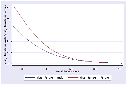
Since this model has multiple outcomes, we need to use the outcome option to indicate which outcome we want to graph when we use postgr3. Below we graph the first outcome (readcat=1).
postgr3 socst, by(female) outcome(1)

Variables left asis: socst _Ifemale_1 _IfemXsocst_1
Holding science constant at 51.85
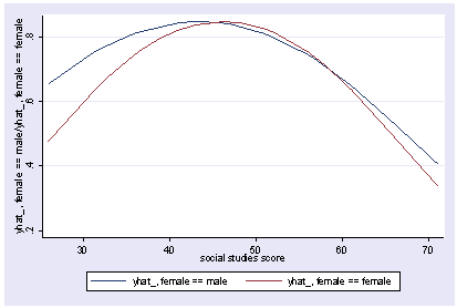
and we show the graph for readcat=2.
postgr3 socst, by(female) outcome(2)

Variables left asis: socst _Ifemale_1 _IfemXsocst_1
Holding science constant at 51.85
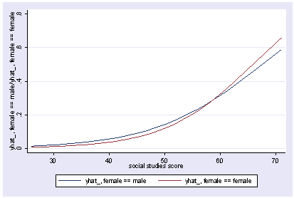
and we show the graph for readcat=3.
postgr3 socst, by(female) outcome(3)

Variables left asis: socst _Ifemale_1 _IfemXsocst_1
Holding science constant at 51.85
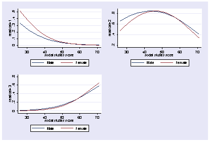
We can show these graphs as one graph like this.
postgr3 socst, by(female) outcome(1) y title("readcat=1") ///
  legend(order(1 "Male" 2 "Female)) saving(g1)

Variables left asis: socst _Ifemale_1 _IfemXsocst_1
Holding science constant at 51.85

<graph omitted to save space>

postgr3 socst, by(female) outcome(2) ytitle("readcat=2") ///
  legend(order(1 "Male" 2 "Female)) saving(g2)

Variables left asis: socst _Ifemale_1 _IfemXsocst_1
Holding science constant at 51.85

<graph omitted to save space>

postgr3 socst, by(female) outcome(2) ytitle("readcat=3") ///
  legend(order(1 "Male" 2 "Female)) saving(g3)

Variables left asis: socst _Ifemale_1 _IfemXsocst_1
Holding science constant at 51.85

<graph omitted to save space>
We can then use graph using to show all 3 graphs together.
graph combine g1.gph g2.gph g3.gph
We would use a similar strategy if we had used mlogit.
The use of postgr3 is also possible for an estimation command like quantile regression. Below we run qreg predicting the median reading score.
xi3: qreg read i.ses*i.female science

i.ses             _Ises_1-3           (naturally coded; _Ises_1 omitted)
i.female          _Ifemale_0-1        (naturally coded; _Ifemale_0 omitted)
i.ses*i.female    _IsesXfem_#_#       (coded as above)
Iteration  1:  WLS sum of weighted deviations =  1256.0231

Iteration  1: sum of abs. weighted deviations =     1253.2
Iteration  2: sum of abs. weighted deviations =     1253.2
Iteration  3: sum of abs. weighted deviations =     1251.6
Iteration  4: sum of abs. weighted deviations =     1246.8
note:  alternate solutions exist
Iteration  5: sum of abs. weighted deviations =       1246
Iteration  6: sum of abs. weighted deviations =       1246
Iteration  7: sum of abs. weighted deviations =       1246

Median regression                                    Number of obs =       200
  Raw sum of deviations     1684 (about 50)
  Min sum of deviations     1246                     Pseudo R2     =    0.2601

------------------------------------------------------------------------------
        read |      Coef.   Std. Err.      t    P>|t|     [95% Conf. Interval]
-------------+----------------------------------------------------------------
     _Ises_2 |       -1.6   4.074188    -0.39   0.695     -9.63565    6.435649
     _Ises_3 |        1.6   4.329626     0.37   0.712    -6.939458    10.13946
  _Ifemale_1 |       -1.8   4.295426    -0.42   0.676      -10.272    6.672005
_IsesXfe~2_1 |        1.8   5.128867     0.35   0.726    -8.315826    11.91583
_IsesXfe~3_1 |        1.8   5.572955     0.32   0.747    -9.191716    12.79172
     science |         .6   .1008242     5.95   0.000     .4011412    .7988588
       _cons |       21.8    6.08162     3.58   0.000     9.805028    33.79497
------------------------------------------------------------------------------
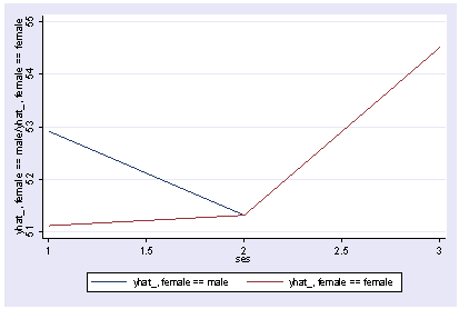
We can show the predicted medians by ses and female as shown below.
postgr3 ses, by(female)

Variables left asis: _Ises_2 _Ises_3 _Ifemale_1 _IsesXfem_2_1 _IsesXfem_3_1
Holding science constant at 51.85

