Purpose: The purpose of this program is to illustrate the central limit theorem. The user may select the type of distribution, the number per sample and the number of samples. Several display options are also available.
Download: You can download this program from within Stata by typing search clt (see How can I use the search command to search for programs and get additional help? for more information about using search).
Use of program: To use this program, type clt in the Stata command window. This opens a dialogue window with numerous pull-down menus, check boxes and buttons. The first pull-down menu allows the user to select the type of distribution: normal, log-normal, exponential, bimodal, binomial or uniform. If binomial is selected, a pull-down menu allows the user to select the probability. Pull-down menus also allow the user to select the number (N) per sample and the number of samples. Four check boxes allow the user to modify the graph that will be displayed by 1) showing a normal curve overlaid on the histogram, 2) draw lines at one and two standard deviations above and below the mean, 3) show the means as z-scores and 4) show sums instead of means. This last option is useful when working with a binomial distribution. Another check box has the program show the distribution being built (i.e., animating the building of the histogram). A pull-down menu allows the user to control the speed of the frames of the animation. This can be done by clicking on the down-arrow to the right of "delay between steps = ". The higher the number, the slower the animation. Once all of the selections have been made, click on the "show" button to view the resulting histogram. To exit the program, click on the "done" button.
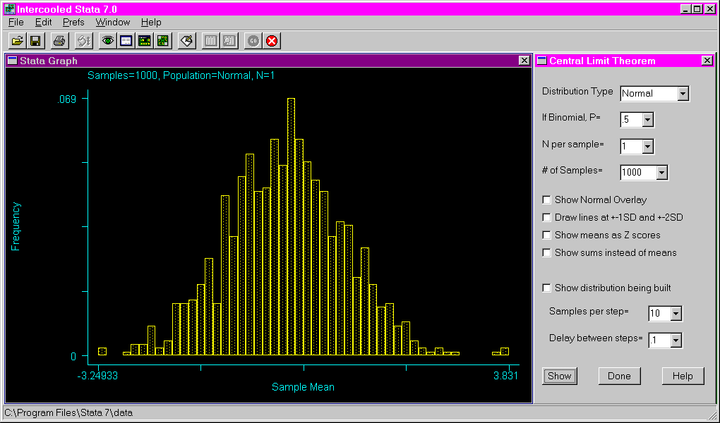
Examples: The following example shows the dialogue window that opens after issuing the clt command and the resulting histogram if only the "show" button is pressed without altering any of the default settings.

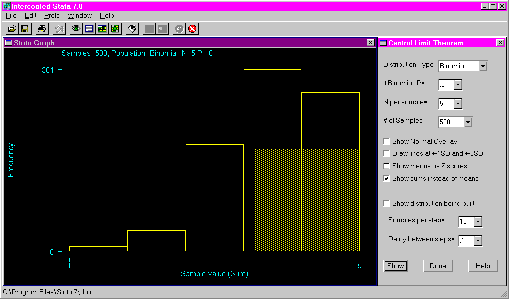
The following shows the results of requesting a binomial distribution with a probability of .8, using a sample size of five and 500 samples. Note that the sums are used on the X axis instead of the means.

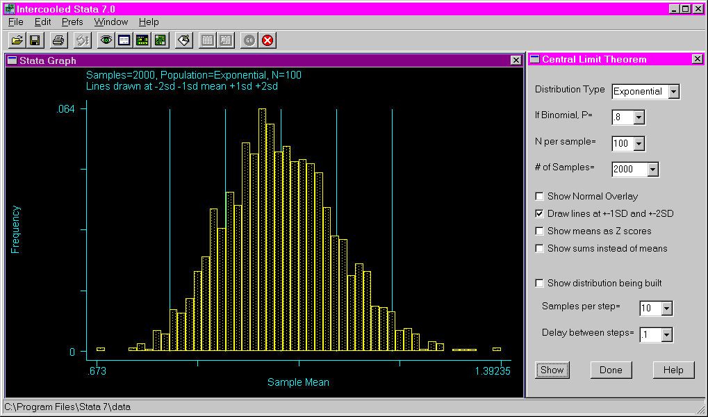
The following shows the results of requesting an exponential distribution with a sample size of 100 and 2000 samples. Lines are drawn at the mean, as well as one and two standard deviations above and below the mean.

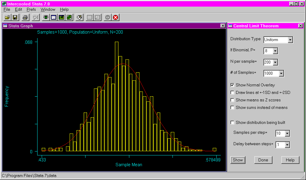
The following shows the results of requesting a uniform distribution with a sample size of 200, 1000 samples and a normal curve overlaid on the graph.

