Version info: Code for this page was tested in Stata 12.1.
This code fragment page shows an example using Mata to write a function that calculates adjusted values from a cox proportional hazards model fit using stcox.
* set up from a Stata example
webuse cancer, clear
stset study died

     failure event:  died != 0 & died < .
obs. time interval:  (0, studytime]
 exit on or before:  failure

------------------------------------------------------------------------------
       48  total obs.
        0  exclusions
------------------------------------------------------------------------------
       48  obs. remaining, representing
       31  failures in single record/single failure data
      744  total analysis time at risk, at risk from t =         0
                             earliest observed entry t =         0
                                  last observed exit t =        39
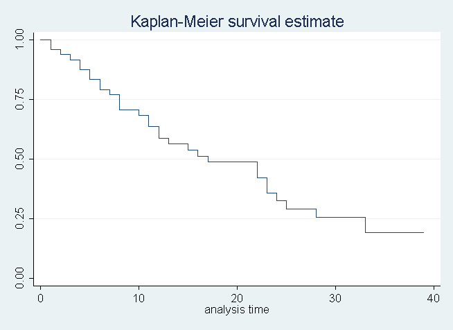
The cox model is a semi-parametric model in that there is a baseline hazard function that is estimated non parametrically and then adjustments based on the covariates are done paramterically. Speicifically, let the unconditional hazard function be the Kaplan-Meier estimate, which in the cox model framework, we denote (lambda_0) to indicate it is the baseline or reference. [ lambda_{0}(t) = prod_{t_{i} < t} frac{n_i - d_i}{n_i} ] which could look like this for example:
sts graph
Now the conditional hazard function for the cox model is [ lambda(t|mathbf{X}) = lambda_{0}(t)e^{mathbf{Xb}} ] where (t) is an n x 1 time vector, (mathbf{X}) is an n x k matrix of predictors and (mathbf{b}) is a k x 1 parameter vector (the estimates from the cox model).
/*
  the model we will fit here time is something other than age,
  age is just a covariate we get coefficients
  (with no hazard ratios) and store the baseline
  hazard function in km for use in getting predicted lines
*/
stcox age i.drug, nohr basesurv(km)

         failure _d:  died
   analysis time _t:  studytime

Iteration 0:   log likelihood = -99.911448
Iteration 1:   log likelihood = -82.331523
Iteration 2:   log likelihood = -81.676487
Iteration 3:   log likelihood = -81.652584
Iteration 4:   log likelihood = -81.652567
Refining estimates:
Iteration 0:   log likelihood = -81.652567

Cox regression -- Breslow method for ties

No. of subjects =           48                     Number of obs   =        48
No. of failures =           31
Time at risk    =          744
                                                   LR chi2(3)      =     36.52
Log likelihood  =   -81.652567                     Prob > chi2     =    0.0000

------------------------------------------------------------------------------
          _t |      Coef.   Std. Err.      z    P>|z|     [95% Conf. Interval]
-------------+----------------------------------------------------------------
         age |     .11184   .0365789     3.06   0.002     .0401467    .1835333
             |
        drug |
          2  |   -1.71156   .4943639    -3.46   0.001    -2.680495   -.7426241
          3  |  -2.956384   .6557432    -4.51   0.000    -4.241617   -1.671151
------------------------------------------------------------------------------
We will not go into the details of estimation or the (partial) likelihood functions for cox models, but from what we have shown, it is evident that in order to calculate the predicted or adjusted hazard functions, we will need three things. First, we need the baseline hazard function, (lambda_0), second we need the parameter vector (mathbf{b}), and finally we need the data values to adjust to, (mathbf{X}). In addition to fitting the model, we extracted and stored the baseline hazard in the variable km with the argument basesurv(km).
As it turns out, the latter two can both be obtained using Stata's margins command which for specific values of the model variables, will give you (mathbf{Xb}) so we do not need to manually calculate the linear predictor.
/*
  use the margins command to get the linear predictions (xb)
  and post them to e(b), these are used by the mata function coxAdjust()
  note it is easist to get all margins of interest at once
*/
margins, at(age=(30(10)80) drug=(1 2 3)) predict(xb) post vsquish

Adjusted predictions                              Number of obs   =         48
Model VCE    : OIM

Expression   : Linear prediction, predict(xb)
1._at        : age             =          30
               drug            =           1
2._at        : age             =          30
               drug            =           2
3._at        : age             =          30
               drug            =           3
4._at        : age             =          40
               drug            =           1
5._at        : age             =          40
               drug            =           2
6._at        : age             =          40
               drug            =           3
7._at        : age             =          50
               drug            =           1
8._at        : age             =          50
               drug            =           2
9._at        : age             =          50
               drug            =           3
10._at       : age             =          60
               drug            =           1
11._at       : age             =          60
               drug            =           2
12._at       : age             =          60
               drug            =           3
13._at       : age             =          70
               drug            =           1
14._at       : age             =          70
               drug            =           2
15._at       : age             =          70
               drug            =           3
16._at       : age             =          80
               drug            =           1
17._at       : age             =          80
               drug            =           2
18._at       : age             =          80
               drug            =           3

------------------------------------------------------------------------------
             |            Delta-method
             |     Margin   Std. Err.      z    P>|z|     [95% Conf. Interval]
-------------+----------------------------------------------------------------
         _at |
          1  |     3.3552   1.097367     3.06   0.002       1.2044    5.505999
          2  |    1.64364   1.091048     1.51   0.132    -.4947747    3.782055
          3  |   .3988159   1.163443     0.34   0.732    -1.881491    2.679123
          4  |     4.4736   1.463156     3.06   0.002     1.605867    7.341332
          5  |    2.76204   1.428609     1.93   0.053     -.037981    5.562062
          6  |   1.517216   1.482118     1.02   0.306    -1.387682    4.422114
          7  |      5.592   1.828945     3.06   0.002     2.007334    9.176666
          8  |    3.88044   1.777375     2.18   0.029     .3968494    7.364031
          9  |   2.635616   1.818612     1.45   0.147    -.9287983     6.20003
         10  |     6.7104   2.194734     3.06   0.002     2.408801      11.012
         11  |    4.99884   2.131855     2.34   0.019     .8204819    9.177199
         12  |   3.754016   2.164631     1.73   0.083    -.4885838    7.996615
         13  |     7.8288   2.560523     3.06   0.002     2.810268    12.84733
         14  |    6.11724   2.489608     2.46   0.014     1.237697    10.99678
         15  |   4.872416    2.51625     1.94   0.053    -.0593427    9.804174
         16  |     8.9472   2.926311     3.06   0.002     3.211735    14.68266
         17  |    7.23564   2.849403     2.54   0.011     1.650913    12.82037
         18  |   5.990816    2.87141     2.09   0.037     .3629549    11.61868
------------------------------------------------------------------------------
We post the output of margins so it is available for later use. Essentially, all that margins is doing is using the values we specified to create a new data matrix, (mathbf{X}) and then post multiplying it by the paramter vector (mathbf{b}) from our model and returning the results. Thus margins returns a p x 1 vector we will call (mathbf{hat{y}}) each element of which corresponds to the particular combination of covariates stored in the corresponding row of (mathbf{X}). Each element of (mathbf{hat{y}}) can be used to create adjusted hazard functions, [ lambda(t|mathbf{X})_{i} = lambda_{0}(t)e^{mathbf{hat{y}_{i}}} ] where (i = 1, ldots, p). This is easy to do all at once in Mata, Stata's matrix programming language. In order to find the median time of survival for a particular adjusted hazard function, let the set be (A) we seek [ min {t cap A < .5} ] of course if (A < .5 = varnothing ) we know that the intersection of (t) and (A < .5) will also be the empty set and the minimum will be undefined, hence left blank. In this situation, one could, perhaps, adjust the probability to another number such that (A < p neq varnothing ) but this code does not. Below we create a Mata function to compute and return (min {t cap A < p}) where (A) is the adjusted hazard function (or functions if you adjust at multiple different values) and (p) is the probability, .5 for median, used as a cut off.
/*
  create a mata function, coxAdjust()
  the first argument is the variable name with the baseline hazard function
  the second argument is the probablility cutoff, such as .5
  although valid values range from 0 to 1
  the third argument is optional and is the base variable name
  used to store the adjusted hazard functions, if blank only the
  values of interest are returned, not the entire adjusted hazard function
*/
mata
real matrix coxAdjust(string scalar baseline, real scalar p, | string scalar basevname)
{
  xb = exp(st_matrix("e(b)"))
  time = st_data(., "_t")
  lambda = log(st_data(., baseline))
  results = exp(lambda * xb)
  if (args()==3) {
    for (i=1; i<=cols(results); i++) {
	  newvar = basevname + strofreal(i)
	  index = st_addvar("double", newvar)
	  st_store((1, rows(results)), index, results[, i])
	}
  }

  tres = J(1, cols(results), .)
  for (i=1; i<=cols(results);i++) {
    tmp = select((time, results[, i]), results[, i] :< p)
	tres[i] = colmin(tmp[,1])
  }
  return(tres)
}
end
Now we can use this to get our median survival times.
/*
  call the coxAdjust() function
  note only the required arguments are used
  the median adjusted survival time are returned and nothing else
*/
mata coxAdjust("km", .5)

       1    2    3    4    5    6    7    8    9   10   11   12   13   14   15   16   17   18
    +-------------------------------------------------------------------------------------------+
  1 |  33    .    .   23    .    .   12   25    .    6   17   25    3    8   22    1    4   10  |
    +-------------------------------------------------------------------------------------------+


* we could get other values
mata coxAdjust("km", .25)

       1    2    3    4    5    6    7    8    9   10   11   12   13   14   15   16   17   18
    +-------------------------------------------------------------------------------------------+
  1 |   .    .    .   25    .    .   22   33    .   10   23    .    5   13   23    2    6   15  |
    +-------------------------------------------------------------------------------------------+

mata coxAdjust("km", .75)

        1    2    3    4    5    6    7    8    9   10   11   12   13   14   15   16   17   18
    +-------------------------------------------------------------------------------------------+
  1 |  23    .    .   13   28    .    7   22   28    4   11   22    1    5   11    1    2    5  |
    +-------------------------------------------------------------------------------------------+

* if instead of just having the medians, we wanted the
* entire hazard functions (e.g., to graph) use the optional argument

mata coxAdjust("km", .5, "p")

       1    2    3    4    5    6    7    8    9   10   11   12   13   14   15   16   17   18
    +-------------------------------------------------------------------------------------------+
  1 |  33    .    .   23    .    .   12   25    .    6   17   25    3    8   22    1    4   10  |
    +-------------------------------------------------------------------------------------------+

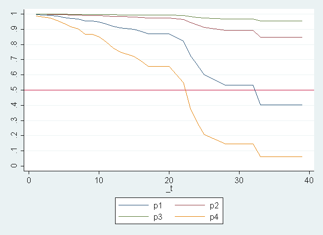
line p1 p2 p3 p4 _t, sort ylab(0(.1)1) xlab(0(10)40) yline(.5)

This graph only includes the first four adjusted survival functions. Corresponding to (mathbf{hat{y}_{i}}) for (i = {1, 2, 3, 4}). These were chosen arbitrary for demonstrative purposes only. The earlier output of the margins command shows us the corresponding values of (mathbf{X}).
Expression   : Linear prediction, predict(xb)
1._at        : age             =          30
               drug            =           1
2._at        : age             =          30
               drug            =           2
3._at        : age             =          30
               drug            =           3
4._at        : age             =          40
               drug            =           1
