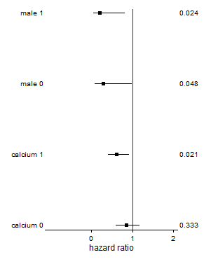
The scheme used for this plot can be downloaded by –search lean scheme– from within Stata. This example has a few steps. The first step is to run all the models and store the parameter estimates and standard errors in a temporary file. The next step is to open the temporary file as a data set and compute the hazard ratio, the confidence interval and its p-value. The last step is to plot them in a compact fashion. The command labmask is part of the labutil ado written by Nicholas J. Cox and can be downloaded via –search labutil-.
use http://www.stata-press.com/data/cgg/hip3, clear

/*creating variable names for the output file*/
capture file close a
file open a using "hr.txt", write replace
file write a "raw_coeff" _tab "stderr" _tab "variable"  _tab "case" _n

/*running separate model on each binary variable and store the estimates*/

foreach var of varlist male calcium {
  tempvar intcat
  gen `intcat' =`var'*protect
  stcox protect `var' `intcat'
  lincom  `var' /*case 0*/
  file write a (`r(estimate)') _tab (`r(se)') _tab ("`var'") _tab (0) _n
  lincom  `var' + `intcat' /*case 1*/
  file write a (`r(estimate)') _tab (`r(se)') _tab ("`var'")  _tab (1) _n

}

file close a

insheet using hr.txt, clear

gen hzratio=exp(raw_coeff)
gen lower=exp(raw_coeff - 1.96*stderr)
gen upper=exp(raw_coeff + 1.96*stderr)

gen p_value = 2*(1-normal(abs(raw_coeff/stderr)))
gen pstring = string(p_value, "%4.3f")

egen group=group(variable case), label

gen group2 = group

labmask group2, values(pstring)

twoway  (scatter group hzratio, msymbol(square)) (rspike lower upper group2, hor yaxis(2)), ///
        legend(off) xline(1, lstyle(refline))  xlabel(0(1) 2) xscale(range(-1 2))  ///
        xtitle(hazard ratio) xsize(4) ylabel(, valuelabel axis(1) tlength(0)) yscale(lstyle(none) axis(1)) ///
        ysize(5) plotregion(style(none)) ylabel(, valuelabel axis(2) tlength(0)) yscale(lstyle(none) axis(2)) ///
        ytitle("", axis(1)) ytitle("", axis(2))  scheme(lean1)

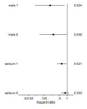
You may prefer to plot the hazard ratios on logarithmically-scaled axes so that the confidence intervals are symmetric. We thank Steven Barger at Northern Arizona University for the suggestion and the code below. Notice the changes to the options xlabel, xscale, and the added option xmtick.
twoway  (scatter group hzratio, msymbol(square)) (rspike lower upper group2, hor yaxis(2)), ///
        legend(off) xline(1, lstyle(refline)) /* new or modifified syntax begins here*/ xmtick(0.0625 0.25) ///
	xlabel(0.03125 .125  .5 1) xscale(log range(0.015625 1.5)) /*ends here*/ ///
        xtitle(hazard ratio) xsize(4) ylabel(, valuelabel axis(1) tlength(0)) yscale(lstyle(none) axis(1)) ///
        ysize(5) plotregion(style(none)) ylabel(, valuelabel axis(2) tlength(0)) yscale(lstyle(none) axis(2)) ///
        ytitle("", axis(1)) ytitle("", axis(2))  scheme(lean1)

