Graphing logistic regression with a continuous variable by continuous variable interaction

This example uses the hsb2 data file to illustrate how to visualize a logistic model with a continuous variable by continuous variable interaction. Variable y is the dependent variable and the predictor variables are read, math, socst and readmath, which is the interaction of read and math.

use https://stats.idre.ucla.edu/stat/stata/notes/hsb2, clear
gen y = (write>60)

gen readmath = read*math
logit y read math  readmath  socst, nolog

Logistic regression                               Number of obs   =        200
                                                  LR chi2(4)      =      66.80
                                                  Prob > chi2     =     0.0000
Log likelihood = -77.953857                       Pseudo R2       =     0.3000

------------------------------------------------------------------------------
           y |      Coef.   Std. Err.      z    P>|z|     [95% Conf. Interval]
-------------+----------------------------------------------------------------
        read |   .4342068   .1961643     2.21   0.027     .0497319    .8186817
        math |   .5104622   .2011857     2.54   0.011     .1161455     .904779
    readmath |  -.0068144   .0033337    -2.04   0.041    -.0133484   -.0002805
       socst |   .0309685   .0271748     1.14   0.254    -.0222931      .08423
       _cons |  -34.09125   11.73402    -2.91   0.004    -57.08951   -11.09299
------------------------------------------------------------------------------

How do we visualize this model? One way to do is to first center the covariates and one of the predictor variable that interacts with the other predictor variable.

sum socst
gen csocst = socst-r(mean)
sum read
gen cread = read-r(mean)
gen creadmath = math*cread

Now we can rerun the model using these variables. Notice that the model is still the same model but parameterized differently.

logit y cread math creadmath csocst, nolog 

Logistic regression                               Number of obs   =        200
                                                  LR chi2(4)      =      66.80
                                                  Prob > chi2     =     0.0000
Log likelihood = -77.953858                       Pseudo R2       =     0.3000

------------------------------------------------------------------------------
           y |      Coef.   Std. Err.      z    P>|z|     [95% Conf. Interval]
-------------+----------------------------------------------------------------
       cread |   .4342067   .1961642     2.21   0.027     .0497319    .8186816
        math |   .1545453   .0390626     3.96   0.000      .077984    .2311067
   creadmath |  -.0068144   .0033337    -2.04   0.041    -.0133484   -.0002805
      csocst |   .0309685   .0271748     1.14   0.254    -.0222931      .08423
       _cons |  -9.789728   2.191172    -4.47   0.000    -14.08435    -5.49511
------------------------------------------------------------------------------

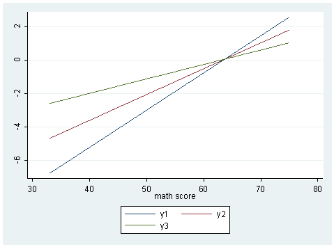
Since cread is a continuous variable, we will have to slice it and see the snapshot at each slice. We will slice it at cread = 0 (corresponding to read equal to its mean), cread = 10 (corresponding to read equal to one standard deviation above the mean) and cread = -10 (corresponding to one standard deviation below the mean), holding math at its particular value and csocst at zero.

gen y1 = _b[_cons] + _b[cread]*(-10) + _b[math]*math  + _b[creadmath]*(-10)*math + _b[csocst]*(0)
gen y2 = _b[_cons] + _b[cread]*(0) + _b[math]*math  + _b[creadmath]*(0)*math + _b[csocst]*(0)
gen y3 = _b[_cons] + _b[cread]*(10) + _b[math]*math  + _b[creadmath]*(10)*math + _b[csocst]*(0)
 
sort math
twoway (line y1 math) (line y2 math) (line y3 math), name(logit, replace)

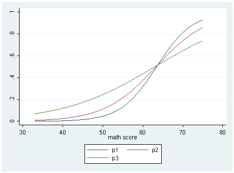
gen p1 = exp(y1)/(1+exp(y1))
gen p2 = exp(y2)/(1+exp(y2))
gen p3 = exp(y3)/(1+exp(y3))

twoway (line p1 math) (line p2 math) (line p3 math), name(prob, replace)