
Version info: Code for this page was tested in Stata 12.
Linear discriminant function analysis (i.e.,
discriminant analysis) performs a multivariate test of differences between
groups. In addition, discriminant analysis is used to determine the
minimum number of dimensions needed to describe these differences. A distinction is sometimes made between descriptive discriminant
analysis and predictive discriminant analysis. We will be illustrating
predictive discriminant analysis on this page.
Please note: The purpose of this page is to show how to use various data
analysis commands. It does not cover all aspects of the research process which
researchers are expected to do. In particular, it does not cover data
cleaning and checking, verification of assumptions, model diagnostics or
potential follow-up analyses.
Examples of discriminant function analysis
Example 1.
A large international air carrier has collected data on employees in three different job
classifications: 1) customer service personnel, 2) mechanics and 3) dispatchers. The director of
Human Resources wants to know if these three job classifications appeal to different personality
types. Each employee is administered a battery of psychological test which include measures
of interest in outdoor activity, sociability and conservativeness.
Example 2.
There is Fisher’s (1936) classic example of discriminant analysis involving three
varieties of iris and
four predictor variables (petal width, petal length, sepal width, and sepal length). Fisher not
only wanted to determine if the varieties differed significantly on the four continuous
variables, but he was also interested in predicting variety classification for unknown individual
plants.
Description of the data
Let’s pursue Example 1 from above.
We have a data file, discrim.dta, with 244 observations on four variables. The psychological variables are outdoor interests, social and
conservative. The categorical variable is job type with three
levels; 1) customer service, 2) mechanic and 3) dispatcher.
Let’s look at the data. It is always a good idea to start with descriptive
statistics.
use https://stats.idre.ucla.edu/stat/stata/dae/discrim, clear

summarize outdoor social conservative

    Variable |       Obs        Mean    Std. Dev.       Min        Max
-------------+--------------------------------------------------------
     outdoor |       244    15.63934    4.839933          0         28
      social |       244    20.67623    5.479262          7         35
conservative |       244    10.59016    3.726789          0         20

tabstat outdoor social conservative, by(job) stat(n mean sd min max) col(stat)

Summary for variables: outdoor social conservative
     by categories of: job

             job |         N      mean        sd       min       max
-----------------+--------------------------------------------------
customer service |        85  12.51765  4.648635         0        22
                 |        85  24.22353  4.335283        12        35
                 |        85  9.023529  3.143309         2        17
-----------------+--------------------------------------------------
        mechanic |        93  18.53763  3.564801        11        28
                 |        93  21.13978   4.55066         9        29
                 |        93  10.13978  3.242354         0        17
-----------------+--------------------------------------------------
        dispatch |        66  15.57576  4.110252         4        25
                 |        66  15.45455  3.766989         7        26
                 |        66  13.24242   3.69224         4        20
-----------------+--------------------------------------------------
           Total |       244  15.63934  4.839933         0        28
                 |       244  20.67623  5.479262         7        35
                 |       244  10.59016  3.726789         0        20
--------------------------------------------------------------------

correlate outdoor social conservative
(obs=244)

             |  outdoor   social conser~e
-------------+---------------------------
     outdoor |   1.0000
      social |  -0.0713   1.0000
conservative |   0.0794  -0.2359   1.0000

tabulate job

             job |      Freq.     Percent        Cum.
-----------------+-----------------------------------
customer service |         85       34.84       34.84
        mechanic |         93       38.11       72.95
        dispatch |         66       27.05      100.00
-----------------+-----------------------------------
           Total |        244      100.00
Analysis methods you might consider
Below is a list of some analysis methods you may have
encountered. Some of the methods listed are quite reasonable, while others
have either fallen out of favor or have limitations.
- Discriminant function analysis – The focus of this page. This procedure is multivariate and also
provides information on the individual dimensions. - Multinomial logistic regression or multinomial probit – These are also viable options.
- MANOVA – The tests of significance are the same as for discriminant function
analysis, but MANOVA gives no information on the individual dimensions.
However, the psychological variables will be the dependent variables and job
type the independent variable. - Separate one-way ANOVAs – You could analyze these data using separate one-way
ANOVAs for each psychological variable. The separate ANOVAs
will not produce multivariate results and do not report information
concerning dimensionality. Again, the designation of independent and
dependent variables is reversed as in MANOVA.
Discriminant function analysis
We will run the discriminant analysis using the candisc procedure. We could also have run the discrim lda command to get the same analysis with slightly
different output. There is a great deal of output, so we will comment at various places
along the way.
candisc outdoor social conservative, group(job)

Canonical linear discriminant analysis

      |                                 | Like-
      | Canon.   Eigen-     Variance    | lihood
  Fcn | Corr.    value   Prop.   Cumul. | Ratio     F      df1    df2  Prob>F
  ----+---------------------------------+------------------------------------
    1 | 0.7207  1.08053  0.7712  0.7712 | 0.3640  52.382     6    478  0.0000 e
    2 | 0.4927  .320504  0.2288  1.0000 | 0.7573   38.46     2    240  0.0000 e
  ---------------------------------------------------------------------------
  Ho: this and smaller canon. corr. are zero;                     e = exact F
- The number of discriminant dimensions is the number of groups minus 1.
However, some discriminant dimensions may not be statistically significant. - In this example, there are two discriminant dimensions, both of which are statistically significant.
The first F-ratio tests that both canonical correlations are zero; the
second F-ratio test that only the second canonical correlation is zero.
Since both of these tests are significant, it follows that both dimensions
are significant and are needed to describe the differences between the three
groups of employees. - The
canonical correlations for the dimensions one and two are 0.72 and 0.49, respectively.
Standardized canonical discriminant function coefficients

                 | function1  function2
    -------------+----------------------
         outdoor |  .3785725   .9261104
          social | -.8306986   .2128593
    conservative |  .5171682  -.2914406

Canonical structure

                 | function1  function2
    -------------+----------------------
         outdoor |  .3230982   .9372155
          social | -.7653907   .2660298
    conservative |   .467691  -.2587426
-
- The standardized discriminant coefficients function in a manner analogous to standardized
regression coefficients in OLS regression. For example, a one standard deviation increase
on the outdoor variable will result in a .3786 standard deviation
increase in the predicted
values on discriminant function 1. - The canonical structure, also known as canonical loading or
discriminant loadings, represent correlations between observed variables and the unobserved
discriminant functions (dimensions). The discriminant functions are a kind of latent variable
and the correlations are loadings analogous to factor loadings.
- The standardized discriminant coefficients function in a manner analogous to standardized
Group means on canonical variables

            | job
    --------+------------------
     group1 | customer service
     group2 | mechanic
     group3 | dispatch

                 | function1  function2
    -------------+----------------------
          group1 |   -1.2191  -.3890039
          group2 |  .1067246   .7145704
          group3 |  1.419669  -.5059049

Resubstitution classification summary

    +---------+
    | Key     |
    |---------|
    | Number  |
    | Percent |
    +---------+
                 | Classified
    True         | group1  group2  group3 |  Total
    -------------+------------------------+-------
          group1 |     70      11       4 |     85
                 |  82.35   12.94    4.71 | 100.00
                 |                        |
          group2 |     16      62      15 |     93
                 |  17.20   66.67   16.13 | 100.00
                 |                        |
          group3 |      3      12      51 |     66
                 |   4.55   18.18   77.27 | 100.00
    -------------+------------------------+-------
           Total |     89      85      70 |    244
                 |  36.48   34.84   28.69 | 100.00
                 |                        |
          Priors | 0.3333  0.3333  0.3333 |
The output includes the means on the discriminant functions for each of the three groups
and a classification table. Values in the diagonal of the classification table reflect
the correct classification of individuals into groups based on their scores on the
discriminant dimensions.
By default, Stata assumes a priori an equal number of people in each
job. This is represented by the 0.3333 Priors in the table above. If
you have different expected proportions in mind, you may specify them with the
priors option.
Next, we will plot a graph of individuals on the discriminant dimensions. Due to the
large number of subjects we will shorten the labels for the job groups to make the
graph more legible. As long as we do not save the dataset, these new labels will not be
made permanent.
label define job 1 "c" 2 "m" 3 "d", modify

scoreplot, msymbol(i)
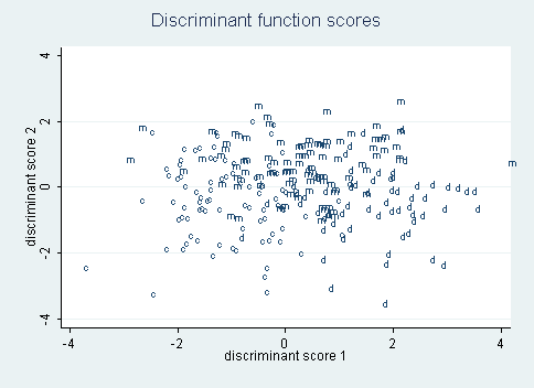
The discrimant functions are:
discriminant_score_1 = 0.517*conservative + 0.379*outdoor – 0.831*social.
discriminant_score_2 = 0.926*outdoor + 0.213*social – 0.291*conservative.
As you can see, the customer service employees tend to be at the more social (negative) end
of dimension 1; the dispatchers are at the opposite end; the mechanics are in the middle. On
dimension 2 the results are not as clear; however, the mechanics tend to be higher on the
outdoor dimension and customer service employees and dispatchers are lower.
We can also plot the discriminant loadings for the variables onto the discriminant
dimensions.
loadingplot
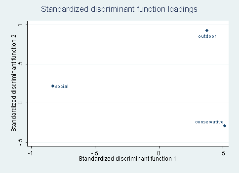
There is no surprise that the variable social is strong on the social dimension, i.e.,
it has a high negative loading, and the outdoor variable is high on the outdoor dimension.
Things to consider
- Multivariate normal distribution assumptions holds for the response variables.
This means that each of the dependent variables is normally distributed
within groups,
that any linear combination of the dependent variables is normally
distributed, and that all subsets of the variables must be multivariate
normal. - Each group must have a sufficiently large number of cases.
- Different classification methods may be used depending on whether the
variance-covariance matrices are equal (or very similar) across groups. - Non-parametric discriminant function analysis, called kth
nearest neighbor, can also be performed.
See also
References
- Grimm, L. G. and Yarnold, P. R. (editors). (1995). Reading
and Understanding Multivariate Statistics. Washington, D.C.:
American Psychological Association. - Huberty, C. J. and Olejnik, S. (2006). Applied MANOVA and
Discriminant Analysis, Second Edition. Hoboken, New Jersey: John
Wiley and Sons, Inc. - Stevens, J. P. (2002). Applied Multivariate Statistics for
the Social Sciences, Fourth Edition. Mahwah, New Jersey:
Lawrence Erlbaum Associates, Inc. - Tatsuoka, M. M. (1971). Multivariate Analysis:
Techniques for Educational and Psychological Research. New York:
John Wiley and Sons.