Hypothetical Scenarios
Example 1
You are interested in studying drinking behavior among adults. Rather than conceptualizing drinking behavior as a continuous variable, you conceptualize it as forming distinct categories or typologies. For example, you think that people fall into one of three different types: abstainers, social drinkers and those who may have a problem with alcohol. Since you cannot directly measure what category someone falls into, this is a latent variable (a variable that cannot be directly measured). However, you do have a number of indicators that you believe are useful for categorizing people into these different categories. Using these indicators, you would like to:
Create a model that permits you to categorize these people into three different types of drinkers, hopefully fitting your conceptualization that there are abstainers, social drinkers and those who may have a problem with alcohol. Be able to categorize people as to what kind of drinker they are. Determine whether three latent classes is the right number of classes (i.e., are there only two types of drinkers or perhaps are there as many as four types of drinkers).
Example 2
High school students vary in their success in school. This might be indicated by the grades one gets, the number of absences one has, the number of truancies one has, and so forth. A traditional way to conceptualize this might be to view “degree of success in high school” as a latent variable (one that you cannot directly measure) that is normally distributed. However, you might conceptualize some students who are struggling and having trouble as forming a different category, perhaps a group you would call “at risk” (or in older days they would be called “juvenile delinquents”). Using indicators like grades, absences, truancies, tardies, suspensions, etc., you might try to identify latent class memberships based on high school success.
Data Description
Let’s pursue Example 1 from above. We have a hypothetical data file that we created that contains 9 fictional measures of drinking behavior. For each measure, the person would be asked whether the description applies to him/herself (yes or no). The 9 measures are
I like to drink I drink hard liquor I have drank in the morning I have drank at work I drink to get drunk I like the taste of alcohol I drink help me sleep Drinking interferes with my relationships I frequently visit bars
We have made up data for 1000 respondents and stored the data in a file called lca1, which is a Stata data file with the subject ID followed by the responses to the 9 questions, coded 1 for yes and 0 for no. The data for the first 10 observations look like this:
list id item1-item9 in 1/10

     +-----------------------------------------------------------------------------+
     |  id   item1   item2   item3   item4   item5   item6   item7   item8   item9 |
     |-----------------------------------------------------------------------------|
  1. | 300       0       0       0       0       0       0       0       0       0 |
  2. | 804       0       0       0       0       0       0       0       0       0 |
  3. | 949       0       0       0       0       0       0       0       0       0 |
  4. |  11       0       0       0       0       0       0       0       0       0 |
  5. | 166       0       0       0       0       0       0       0       0       0 |
     |-----------------------------------------------------------------------------|
  6. | 269       0       0       0       0       0       0       0       0       0 |
  7. | 437       0       0       0       0       0       0       0       0       0 |
  8. | 678       0       0       0       0       0       0       0       0       0 |
  9. | 379       0       0       0       0       0       0       0       0       0 |
 10. | 525       0       0       0       0       0       0       0       0       0 |
     +-----------------------------------------------------------------------------+
Some Strategies You Might Try
Before we show how you can analyze this with Latent Class Analysis, let’s consider some other methods that you might use:
Cluster Analysis – You could use cluster analysis for data like these. However, cluster analysis is not based on a statistical model. It can tell you how the cases are clustered into groups, but it does not provide information such as the probability that a given person is an alcoholic or abstainer. Also, cluster analysis would not provide information such as: given that someone said “yes” to drinking at work, what is the probability that they are an alcoholic. Factor Analysis – Because the term “latent variable” is used, you might be tempted to use factor analysis, since that is a technique used with latent variables. However, factor analysis is used for continuous and usually normally distributed latent variables, where this latent variable, e.g., alcoholism, is categorical.
Latent Class Analysis
Stata’s gsem is used to run a latent class analysis. After the command, the categorical predictor variables are listed. Because the variables in this example are numbered consecutively from 1 to 9, we can simply list the first variable name, item1, followed by a dash, and then the last variable name, item9. This is followed by an arrow pointing toward the predictors. The _cons is optional; the analysis will run if it is there are not. After closing the parentheses, a comma is given, indicating that options will follow. We list the family as bernoulli, the link as logit (because our predictors are binary), and then use the lclass option. In the parentheses, we give the name of the class, usually an upper-case C, and the number of classes we want.
gsem (item1-item9 <- _cons), family(bernoulli) link(logit) lclass(C 3)
Fitting class model:

Iteration 0:  (class) log likelihood = -1098.6113
Iteration 1:  (class) log likelihood = -1098.6113

Fitting outcome model:

Iteration 0:  (outcome) log likelihood = -3758.2924
Iteration 1:  (outcome) log likelihood = -3646.4855
Iteration 2:  (outcome) log likelihood = -3630.2169
Iteration 3:  (outcome) log likelihood = -3626.9688
Iteration 4:  (outcome) log likelihood = -3626.3104
Iteration 5:  (outcome) log likelihood = -3626.1551
Iteration 6:  (outcome) log likelihood = -3626.1263
Iteration 7:  (outcome) log likelihood = -3626.1234
Iteration 8:  (outcome) log likelihood = -3626.1228
Iteration 9:  (outcome) log likelihood = -3626.1226
Iteration 10: (outcome) log likelihood = -3626.1226

Refining starting values:

Iteration 0:  (EM) log likelihood = -4931.4182
Iteration 1:  (EM) log likelihood = -4973.2876
Iteration 2:  (EM) log likelihood = -4980.0232
Iteration 3:  (EM) log likelihood = -4975.9769
Iteration 4:  (EM) log likelihood = -4968.4002
Iteration 5:  (EM) log likelihood = -4959.8284
Iteration 6:  (EM) log likelihood = -4951.1641
Iteration 7:  (EM) log likelihood = -4942.6958
Iteration 8:  (EM) log likelihood = -4934.4788
Iteration 9:  (EM) log likelihood = -4926.4841
Iteration 10: (EM) log likelihood = -4918.6582
Iteration 11: (EM) log likelihood = -4910.9457
Iteration 12: (EM) log likelihood = -4903.2977
Iteration 13: (EM) log likelihood = -4895.6746
Iteration 14: (EM) log likelihood = -4888.0454
Iteration 15: (EM) log likelihood = -4880.3882
Iteration 16: (EM) log likelihood =  -4872.689
Iteration 17: (EM) log likelihood = -4864.9418
Iteration 18: (EM) log likelihood = -4857.1472
Iteration 19: (EM) log likelihood = -4849.3128
Iteration 20: (EM) log likelihood = -4841.4511
note: EM algorithm reached maximum iterations.

Fitting full model:

Iteration 0:  Log likelihood = -4243.4772  (not concave)
Iteration 1:  Log likelihood = -4242.3749  (not concave)
Iteration 2:  Log likelihood = -4241.0733  (not concave)
Iteration 3:  Log likelihood = -4240.0798  (not concave)
Iteration 4:  Log likelihood = -4236.6898  (not concave)
Iteration 5:  Log likelihood =  -4236.656  (not concave)
Iteration 6:  Log likelihood = -4234.9869
Iteration 7:  Log likelihood =  -4232.749  (not concave)
Iteration 8:  Log likelihood = -4232.2285
Iteration 9:  Log likelihood = -4231.9255
Iteration 10: Log likelihood = -4231.7821
Iteration 11: Log likelihood = -4231.7411  (not concave)
Iteration 12: Log likelihood =  -4231.702
Iteration 13: Log likelihood = -4231.6959
Iteration 14: Log likelihood = -4231.6958

Generalized structural equation model                    Number of obs = 1,000
Log likelihood = -4231.6958

------------------------------------------------------------------------------
             | Coefficient  Std. err.      z    P>|z|     [95% conf. interval]
-------------+----------------------------------------------------------------
1.C          |  (base outcome)
-------------+----------------------------------------------------------------
2.C          |
       _cons |   .4287798   .8185974     0.52   0.600    -1.175642    2.033201
-------------+----------------------------------------------------------------
3.C          |
       _cons |  -1.521675   .6923291    -2.20   0.028    -2.878615   -.1647353
------------------------------------------------------------------------------

Class:    1

Response: item1
Family:   Bernoulli
Link:     Logit

Response: item2
Family:   Bernoulli
Link:     Logit

Response: item3
Family:   Bernoulli
Link:     Logit

Response: item4
Family:   Bernoulli
Link:     Logit

Response: item5
Family:   Bernoulli
Link:     Logit

Response: item6
Family:   Bernoulli
Link:     Logit

Response: item7
Family:   Bernoulli
Link:     Logit

Response: item8
Family:   Bernoulli
Link:     Logit

Response: item9
Family:   Bernoulli
Link:     Logit

------------------------------------------------------------------------------
             | Coefficient  Std. err.      z    P>|z|     [95% conf. interval]
-------------+----------------------------------------------------------------
item1        |
       _cons |  -.7899339   .9859737    -0.80   0.423    -2.722407    1.142539
-------------+----------------------------------------------------------------
item2        |
       _cons |  -1.628514   .3027822    -5.38   0.000    -2.221956   -1.035071
-------------+----------------------------------------------------------------
item3        |
       _cons |  -3.295288   .4608422    -7.15   0.000    -4.198523   -2.392054
-------------+----------------------------------------------------------------
item4        |
       _cons |  -2.823975   .3176524    -8.89   0.000    -3.446562   -2.201388
-------------+----------------------------------------------------------------
item5        |
       _cons |  -3.069835   .8750441    -3.51   0.000     -4.78489    -1.35478
-------------+----------------------------------------------------------------
item6        |
       _cons |  -1.496508   .3030282    -4.94   0.000    -2.090432   -.9025834
-------------+----------------------------------------------------------------
item7        |
       _cons |  -2.223255   .2496319    -8.91   0.000    -2.712524   -1.733985
-------------+----------------------------------------------------------------
item8        |
       _cons |  -2.091981   .2295699    -9.11   0.000    -2.541929   -1.642032
-------------+----------------------------------------------------------------
item9        |
       _cons |  -1.464306   .2636135    -5.55   0.000    -1.980979   -.9476332
------------------------------------------------------------------------------

Class:    2

Response: item1
Family:   Bernoulli
Link:     Logit

Response: item2
Family:   Bernoulli
Link:     Logit

Response: item3
Family:   Bernoulli
Link:     Logit

Response: item4
Family:   Bernoulli
Link:     Logit

Response: item5
Family:   Bernoulli
Link:     Logit

Response: item6
Family:   Bernoulli
Link:     Logit

Response: item7
Family:   Bernoulli
Link:     Logit

Response: item8
Family:   Bernoulli
Link:     Logit

Response: item9
Family:   Bernoulli
Link:     Logit

------------------------------------------------------------------------------
             | Coefficient  Std. err.      z    P>|z|     [95% conf. interval]
-------------+----------------------------------------------------------------
item1        |
       _cons |   2.292889   1.053674     2.18   0.030     .2277263    4.358053
-------------+----------------------------------------------------------------
item2        |
       _cons |  -.6748749   .2540475    -2.66   0.008    -1.172799    -.176951
-------------+----------------------------------------------------------------
item3        |
       _cons |  -2.637822   .2810791    -9.38   0.000    -3.188727   -2.086917
-------------+----------------------------------------------------------------
item4        |
       _cons |  -2.658283   .3095767    -8.59   0.000    -3.265043   -2.051524
-------------+----------------------------------------------------------------
item5        |
       _cons |  -1.270617   .3102912    -4.09   0.000    -1.878776   -.6624574
-------------+----------------------------------------------------------------
item6        |
       _cons |   -.755464   .1985341    -3.81   0.000    -1.144584   -.3663442
-------------+----------------------------------------------------------------
item7        |
       _cons |  -2.062337   .2129544    -9.68   0.000     -2.47972   -1.644954
-------------+----------------------------------------------------------------
item8        |
       _cons |  -1.816183   .2258445    -8.04   0.000     -2.25883   -1.373536
-------------+----------------------------------------------------------------
item9        |
       _cons |  -.7314625   .1820354    -4.02   0.000    -1.088245   -.3746796
------------------------------------------------------------------------------

Class:    3

Response: item1
Family:   Bernoulli
Link:     Logit

Response: item2
Family:   Bernoulli
Link:     Logit

Response: item3
Family:   Bernoulli
Link:     Logit

Response: item4
Family:   Bernoulli
Link:     Logit

Response: item5
Family:   Bernoulli
Link:     Logit

Response: item6
Family:   Bernoulli
Link:     Logit

Response: item7
Family:   Bernoulli
Link:     Logit

Response: item8
Family:   Bernoulli
Link:     Logit

Response: item9
Family:   Bernoulli
Link:     Logit

------------------------------------------------------------------------------
             | Coefficient  Std. err.      z    P>|z|     [95% conf. interval]
-------------+----------------------------------------------------------------
item1        |
       _cons |   2.487929   .5795831     4.29   0.000     1.351967    3.623891
-------------+----------------------------------------------------------------
item2        |
       _cons |   .1851186   .3154212     0.59   0.557    -.4330956    .8033328
-------------+----------------------------------------------------------------
item3        |
       _cons |  -.2965715   .3835435    -0.77   0.439    -1.048303      .45516
-------------+----------------------------------------------------------------
item4        |
       _cons |  -.3312536   .3358622    -0.99   0.324    -.9895315    .3270242
-------------+----------------------------------------------------------------
item5        |
       _cons |   1.182954   .5570521     2.12   0.034     .0911515    2.274756
-------------+----------------------------------------------------------------
item6        |
       _cons |  -.1160543   .3060531    -0.38   0.705    -.7159073    .4837988
-------------+----------------------------------------------------------------
item7        |
       _cons |   .0495348   .3718233     0.13   0.894    -.6792255    .7782951
-------------+----------------------------------------------------------------
item8        |
       _cons |   .4862054   .4581794     1.06   0.289    -.4118098    1.384221
-------------+----------------------------------------------------------------
item9        |
       _cons |  -.6241858   .3073837    -2.03   0.042    -1.226647   -.0217248
------------------------------------------------------------------------------
Although there is a lot of output, there is not too much you need to do with it. The model needs to be run so that we can then request the latent class probabilities and the latent class means.
Conditional Probabilities
We use the post-estimation command estat lcprob to get the latent class probabilities.
estat lcprob
Latent class marginal probabilities Number of obs = 1,000
--------------------------------------------------------------
| Delta-method
| Margin std. err. [95% conf. interval]
-------------+------------------------------------------------
C |
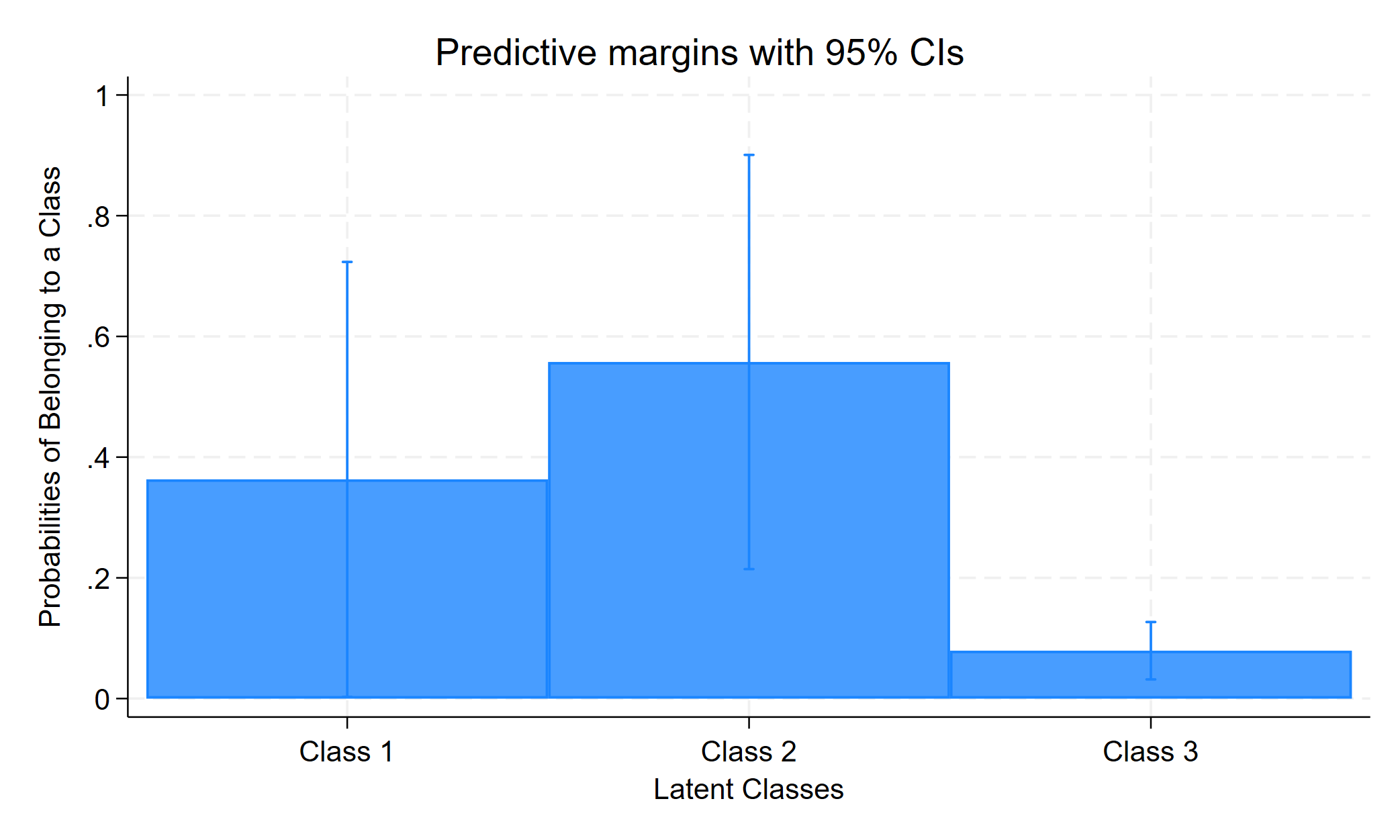
1 | .363144 .1838146 .1072129 .7302799
2 | .5575651 .1750544 .2387489 .8350876
3 | .079291 .0242463 .0429849 .1417209
--------------------------------------------------------------
We see that the average probability of being in latent class 1 is approximately .36; the average probability of being in latent class 2 is approximately .56; and the average probability of being in latent class 3 is 0.08.
The post-estimation command estat lcmean gives the average proportion of endorsement (meaning selecting 1 rather than 0) for each item in each latent class.
estat lcmean
Latent class marginal means                              Number of obs = 1,000

--------------------------------------------------------------
             |            Delta-method
             |     Margin   std. err.     [95% conf. interval]
-------------+------------------------------------------------
1            |
       item1 |   .3121829   .2117129      .0616641    .7581455
       item2 |   .1640341   .0415196      .0977961    .2621021
       item3 |   .0357332   .0158789      .0147956    .0837806
       item4 |   .0560423   .0168043      .0308716     .099626
       item5 |   .0443688   .0371021      .0082858      .20509
       item6 |    .182947   .0452959      .1100302    .2885199
       item7 |   .0976816   .0220025      .0622384    .1500786
       item8 |   .1098787   .0224532      .0729706    .1621888
       item9 |   .1878096   .0402109      .1212145     .279361
-------------+------------------------------------------------
2            |
       item1 |   .9082864   .0877734      .5566868    .9873586
       item2 |   .3374061   .0567957      .2363495    .4558773
       item3 |   .0667436   .0175081      .0395922    .1103749
       item4 |   .0654803   .0189438      .0367901    .1138985
       item5 |   .2191517   .0530983      .1325295    .3401878
       item6 |   .3196319   .0431747      .2414798    .4094247
       item7 |   .1128118   .0213136      .0772922    .1617921
       item8 |   .1398925   .0271742      .0945905    .2020492
       item9 |   .3248739    .039926      .2519488    .4074107
-------------+------------------------------------------------
3            |
       item1 |   .9232913   .0410487       .794451    .9740146
       item2 |   .5461479   .0781836      .3933874    .6906869
       item3 |   .4263958    .093808      .2595511    .6118654
       item4 |   .4179356   .0817037      .2710046    .5810351
       item5 |   .7654785   .1000027      .5227721    .9067646
       item6 |    .471019   .0762562      .3282948    .6186445
       item7 |   .5123812   .0928988      .3364342    .6853126
       item8 |   .6192121   .1080334      .3984782     .799668
       item9 |   .3488301   .0698215      .2267688     .494569
--------------------------------------------------------------
Looking at item1 across the three classes, we see that it was endorsed by a little less than a third of those in latent class 1 and by more than 90% of those in latent classes 2 and 3. Looking at the pattern of responses for each item in each latent class should be helpful in determining the nature of each class. In our example, it seems that those in latent class 1 are those who are “social” drinkers; those in latent class 2 seem to be those who tend to abstain from alcohol, and those in latent class 3 may have a problem with alcohol.
The output above is useful, but it is not in a format that would be easily understood by most audiences. Let’s reformat the output to make it easier to read, as shown below. Each row represents a different item, and the three columns of numbers are the probabilities of answering “yes” to the item given that you belonged to that class. So, if you belong to latent class 1, you have a 90.8% probability of saying “yes, I like to drink”. By contrast, if you belong to latent class 2, you have a 31.2% chance of saying “yes, I like to drink”.
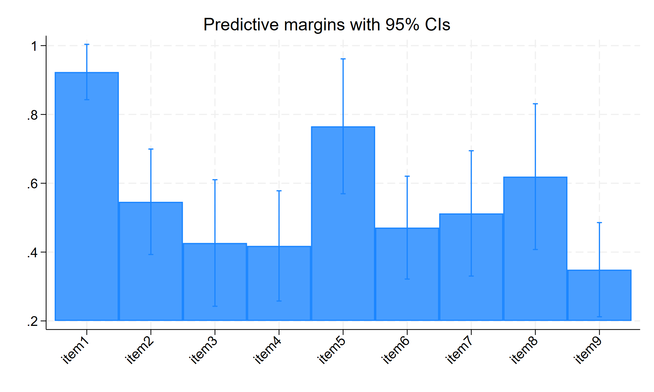
Class 1 Class 2 Class 3 Item Label
ITEM1 0.312 0.908 0.923 I like to drink
ITEM2 0.164 0.337 0.546 I drink hard liquor
ITEM3 0.036 0.067 0.426 I have drank in the morning
ITEM4 0.056 0.065 0.418 I have drank at work
ITEM5 0.044 0.219 0.765 I drink to get drunk
ITEM6 0.183 0.320 0.471 I like the taste of alcohol
ITEM7 0.098 0.113 0.512 I drink help me sleep
ITEM8 0.110 0.140 0.619 Drinking interferes with my relationships
ITEM9 0.188 0.325 0.349 I frequently visit bars
Looking at item1, those in latent class 2 and latent class3 really like to drink (with 90.8% and 92.3% saying yes) while those in latent class1 are not so fond of drinking (they have only a 31.2% probability of saying they like to drink). Jumping to item5, 76.5% of those in latent class 3 say they drink to get drunk, while 21.9% of those in latent class2 agreed to that, and only 4.4% of those in latent class1 say that.
Focusing just on latent class 3 (looking at that column), they really like to drink (92%), they drink hard liquor (54.6%), a pretty large number say they have drank in the morning and at work (42.6% and 41.8%), and well over half say drinking interferes with their relationships (61.9%).
It seems that those in latent class 1 are those who tend to abstain from alcohol; we were expecting to find a latent class like this. Not many of them like to drink (31.2%), few like the taste of alcohol (18.3%), few frequently visit bars (18.8%), and for the rest of the questions they rarely answered “yes”.
This leaves latent class 2; they seem fit the idea of the “social” drinker. They like to drink (90.8%), but they don’t drink hard liquor as often as Class 3 (33.7% versus 54.6%). They rarely drink in the morning or at work (6.7% and 6.5%) and rarely say that drinking interferes with their relationships (14%). They say they frequently visit bars similar to latent class 3 (32.5% versus 34.9%), but that might make sense. Both the social drinkers and those with a problem with alcohol are similar in how much they like to drink and how frequently they go to bars, but differ in key ways such as drinking at work, drinking in the morning, and the impact of drinking on their relationships.
We may also want to know how well this model fits these data, so we can use the post-estimation command estat lcgof.
estat lcgof
----------------------------------------------------------------------------
Fit statistic        |      Value   Description
---------------------+------------------------------------------------------
Likelihood ratio     |
        chi2_ms(482) |    319.955   model vs. saturated
            p > chi2 |      1.000
---------------------+------------------------------------------------------
Information criteria |
                 AIC |   8521.392   Akaike's information criterion
                 BIC |   8663.716   Bayesian information criterion
----------------------------------------------------------------------------
We fail to reject the null hypothesis that the fitted model fits as well as the saturated model.
Graphing the Results
All write-ups of latent class analyses contain tables of results, but graphs are useful as well. In Stata, we use the post-estimation command margins to create a table with particular content, and then use marginsplot to graph the contents of the table. You use must run the margins command before you run the marginsplot command. Let’s start with a basic graph, and then we will modify the graph to make it look nicer.
margins, predict(classpr class(1)) predict(classpr class(2)) predict(classpr class(3))
marginsplot
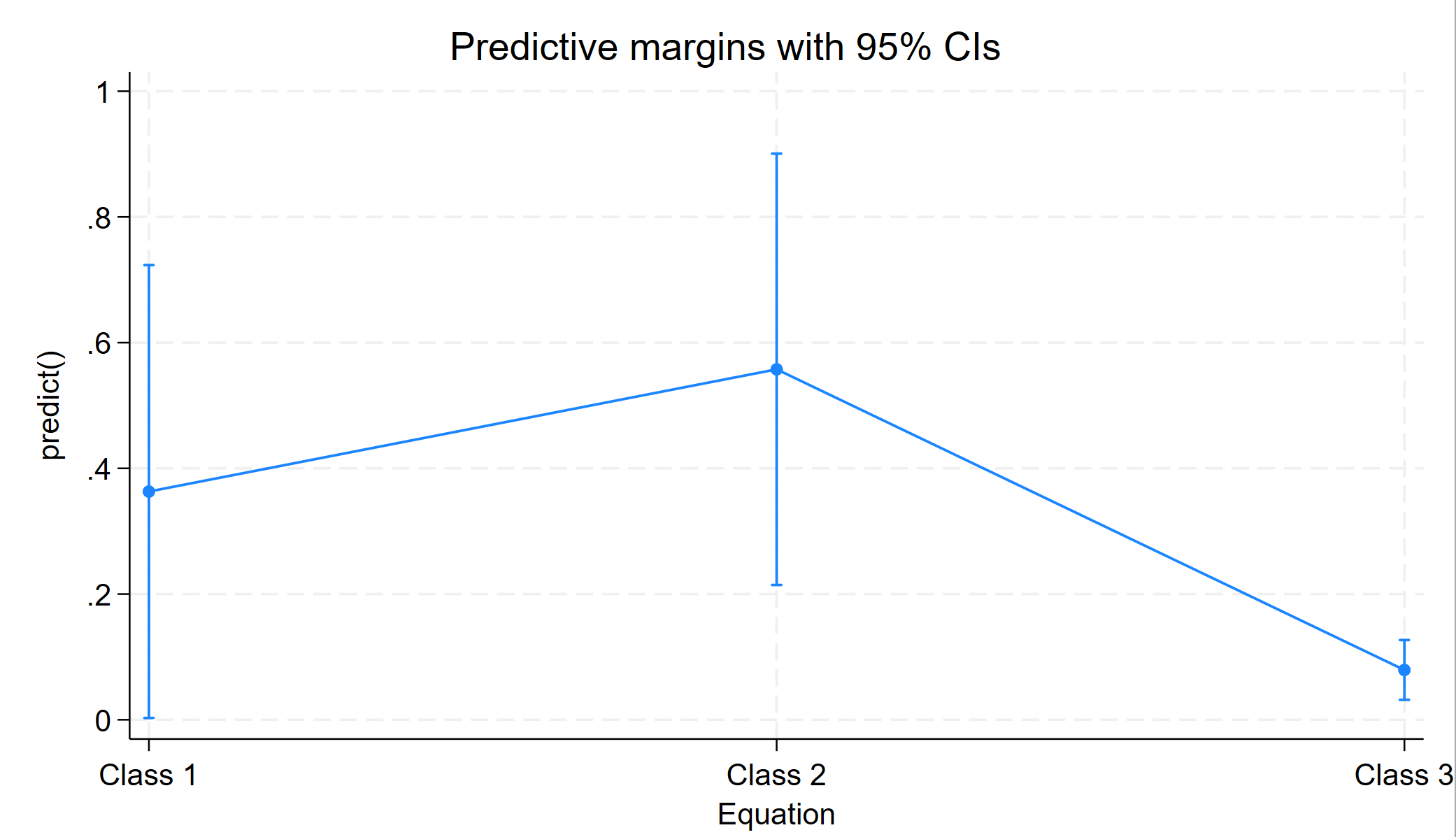
This graph is OK, but it could be better. We will add some options to the marginsplot command to improve the graph. Among other options, we will use the recast option, which changes the graph from a line graph to a bar graph.
marginsplot, recast(bar) xtitle("Latent Classes") ytitle("Probabilities of Belonging to a Class") xlabel(1 "Class 1" 2 "Class 2" 3 "Class 3") title("Predicted Migraine Latent Class Probabilities with 95% CI")
We can also make graphs showing the predicted probabilities for each of the items in our analysis.
margins, predict(outcome(item1) class(3)) predict(outcome(item2) class(3)) predict(outcome(item3) class(3)) predict(outcome(item4) class(3)) predict(outcome(item5) class(3)) predict(outcome(item6) class(3)) predict(outcome(item7) class(3)) predict(outcome(item8) class(3)) predict(outcome(item9) class(3))
marginsplot, recast(bar) xtitle("") ytitle("") xlabel(1 "item1" 2 "item2" 3 "item3" 4 "item4" 5 "item5" 6 "item6" 7 "item7" 8 "item8" 9 "item9", angle(45)) title("Predicted Probability of Behaviors For Class 3 with 95% CI")
Number of Classes
So far we have been assuming that we have chosen the right number of latent classes. Perhaps, however, there are only two types of drinkers, or perhaps there are four or more types of drinkers. So far we have liked the three class model, both based on our theoretical expectations and based on how interpretable our results have been. We can further assess whether we have chosen the right number of classes by running the analysis with different numbers of classes and then comparing the fit of the models. In our example, we may have wanted to compare a one-class, two-class, three-class and four-class model and then compare the results. However, a four-class model will not run with our example data, so we will run a one-class, two-class and three-class model and then compare the results with the estimates stats command. We use the quietly prefix before each gsem command to suppress the output.
quietly gsem (item1-item9 <- ), family(bernoulli) link(logit) lclass(C 1)
estimates store oneclass
quietly gsem (item1-item9 <- ), family(bernoulli) link(logit) lclass(C 2)
estimates store twoclass
quietly gsem (item1-item9 <- ), family(bernoulli) link(logit) lclass(C 3)
estimates store threeclass
* lower is better
estimates stats oneclass twoclass threeclass
Akaike's information criterion and Bayesian information criterion

-----------------------------------------------------------------------------
       Model |          N   ll(null)  ll(model)      df        AIC        BIC
-------------+---------------------------------------------------------------
    oneclass |      1,000          .  -4348.878       9   8715.755   8759.925
    twoclass |      1,000          .  -4251.208      19   8540.416   8633.664
  threeclass |      1,000          .  -4231.696      29   8521.392   8663.716
-----------------------------------------------------------------------------
Note: BIC uses N = number of observations. See [R] IC note.
Both the AIC and BIC are lower for the three-class solution, so we think this is a good model.
Cautions, Flies in the Ointment
We have focused on a very simple example here just to get you started. Here are some problems to watch out for.
Have you specified the right number of latent classes? Perhaps you have specified too many classes (i.e., people largely fall into 2 classes) or you may have specified too few classes (i.e., people really fall into 4 or more classes).
Are some of your measures/indicators lousy? All of our measures were really useful in distinguishing what type of drinker the person was. However, say we had a measure that was “Do you like broccoli?”. This would be a poor indicator, and each type of drinker would probably answer in a similar way, so this question would be a good candidate to discard.
Having developed this model to identify the different types of drinkers, we might be interested in trying to predict why someone is an alcoholic, or why someone is an abstainer. For example, we might be interested in whether parental drinking predicts being an alcoholic. Such analyses are possible but not discussed here.
References
Masyn, Katherine E. Latent Class Analysis and Finite Mixture Modeling. (2013). In The Oxford Handbook of Quantitative Methods. Edited by Todd Little.