Version info: Code for this page was tested in Stata 18
Mixed effects logistic regression is used to model binary outcome variables, in which the log odds of the outcomes are modeled as a linear combination of the predictor variables when data are clustered or there are both fixed and random effects.
Please note: The purpose of this page is to show how to use various data analysis commands. It does not cover all aspects of the research process which researchers are expected to do. In particular, it does not cover data cleaning and checking, verification of assumptions, model diagnostics or potential follow-up analyses.
Examples of mixed effects logistic regression
Example 1: A researcher sampled applications to 40 different colleges to study factors that predict admittance into college. Predictors include student’s high school GPA, extracurricular activities, and SAT scores. Some colleges are more or less selective, so the baseline probability of admittance into each of the colleges is different. College-level predictors include whether the college is public or private, the current student-to-teacher ratio, and the college’s rank.
Example 2: A large HMO wants to know what patient and physician factors are most related to whether a patient’s lung cancer goes into remission after treatment as part of a larger study of treatment outcomes and quality of life in patients with lunge cancer.
Example 3: A television station wants to know how time and advertising campaigns affect whether people view a television show. They sample people from four cities for six months. Each month, they ask whether the people had watched a particular show or not in the past week. After three months, they introduced a new advertising campaign in two of the four cities and continued monitoring whether or not people had watched the show.
Description of the data
In this example, we are going to explore Example 2 about lung cancer using a simulated dataset, which we have posted online. A variety of outcomes were collected on patients, who are nested within doctors, who are in turn nested within hospitals. There are also a few doctor level variables, such as experience, that we will use in our example.
*Grab the most recent version from the internet
insheet using "https://stats.idre.ucla.edu/stat/data/hdp.csv", comma

foreach i of varlist familyhx smokinghx sex cancerstage school {
encode `i', gen(`i'2)
drop `i'
rename `i'2 `i'
}
Here is a general summary of the whole dataset.
summarize
    Variable |       Obs        Mean    Std. Dev.       Min        Max
-------------+--------------------------------------------------------
   tumorsize |      8525    70.88067    12.06833   33.96859   116.4579
         co2 |      8525    1.605207    .1238528   1.222361   2.128112
        pain |      8525    5.473314    1.504302          1          9
       wound |      8525    5.731848    1.525207          1          9
    mobility |      8525    6.080469    1.484188          1          9
-------------+--------------------------------------------------------
     ntumors |      8525    3.066276    2.550696          0          9
   nmorphine |      8525     3.62393    2.503595          0         18
   remission |      8525    .2957185    .4563918          0          1
lungcapacity |      8525    .7740865    .1756213   .0161208   .9997957
         age |      8525    50.97205    6.275041   26.32264   74.48235
-------------+--------------------------------------------------------
     married |      8525          .6    .4899267          0          1
lengthofstay |      8525    5.492199     1.04961          1         10
         wbc |      8525     5997.58    995.1962   2131.302   9776.412
         rbc |      8525    4.995027    .2891493   3.918932    6.06487
         bmi |      8525    29.07269    6.648291   18.38268         58
-------------+--------------------------------------------------------
         il6 |      8525    4.016984    2.858684   .0352107   23.72776
         crp |      8525    4.973017    3.108535   .0451048   28.74212
         did |      8525    203.3309    119.4691          1        407
  experience |      8525    17.64129    4.075327          7         29
    lawsuits |      8525    1.866393    1.486401          0          9
-------------+--------------------------------------------------------
         hid |      8525    17.76422    10.21063          1         35
    medicaid |      8525     .512513    .2072415   .1415814   .8187299
    familyhx |      8525         1.2    .4000235          1          2
   smokinghx |      8525         2.4    .8000469          1          3
         sex |      8525         1.4    .4899267          1          2
-------------+--------------------------------------------------------
 cancerstage |      8525    2.100059    .9436027          1          4
      school |      8525     1.24868    .4322735          1          2
We can also get the frequencies for categorical or discrete variables, and the correlations for continuous predictors.
tab1 remission cancerstage lengthofstay
-> tabulation of remission

  remission |      Freq.     Percent        Cum.
------------+-----------------------------------
          0 |      6,004       70.43       70.43
          1 |      2,521       29.57      100.00
------------+-----------------------------------
      Total |      8,525      100.00

-> tabulation of cancerstage

CancerStage |      Freq.     Percent        Cum.
------------+-----------------------------------
          I |      2,558       30.01       30.01
         II |      3,409       39.99       69.99
        III |      1,705       20.00       89.99
         IV |        853       10.01      100.00
------------+-----------------------------------
      Total |      8,525      100.00

-> tabulation of lengthofstay

LengthofSta |
          y |      Freq.     Percent        Cum.
------------+-----------------------------------
          1 |          2        0.02        0.02
          2 |         14        0.16        0.19
          3 |        181        2.12        2.31
          4 |      1,196       14.03       16.34
          5 |      2,896       33.97       50.31
          6 |      2,874       33.71       84.02
          7 |      1,168       13.70       97.72
          8 |        183        2.15       99.87
          9 |         10        0.12       99.99
         10 |          1        0.01      100.00
------------+-----------------------------------
      Total |      8,525      100.00
cor il6 crp lengthofstay experience
(obs=8,525)

             |      il6      crp length~y experi~e
-------------+------------------------------------
         il6 |   1.0000
         crp |   0.0024   1.0000
lengthofstay |  -0.0066   0.0175   1.0000
  experience |  -0.0039  -0.0052   0.0128   1.0000
Analysis methods you might consider
Below is a list of analysis methods you may have considered.
- Mixed effects logistic regression, the focus of this page.
- Mixed effects probit regression is very similar to mixed effects logistic regression, but it uses the normal CDF instead of the logistic CDF. Both model binary outcomes and can include fixed and random effects.
- Fixed effects logistic regression is limited in this case because it may ignore necessary random effects and/or non independence in the data.
- Fixed effects probit regression is limited in this case because it may ignore necessary random effects and/or non independence in the data.
- Logistic regression with clustered standard errors. These can adjust for non independence but does not allow for random effects.
- Probit regression with clustered standard errors. These can adjust for non independence but does not allow for random effects.
Mixed effects logistic regression
Below we use the melogit command to estimate a mixed effects logistic regression model with il6, crp, and lengthofstay as patient level continuous predictors, cancerstage as a patient level categorical predictor (I, II, III, or IV), experience as a doctor level continuous predictor, and a random intercept by did, doctor ID.
Estimating and interpreting generalized linear mixed models (GLMMs, of which mixed effects logistic regression is one) can be quite challenging. If you are just starting, we highly recommend reading this page first Introduction to GLMMs. It covers some of the background and theory as well as estimation options, inference, and pitfalls in more detail.
melogit remission il6 crp i.cancerstage lengthofstay experience || did:
Fitting fixed-effects model:

Iteration 0:  Log likelihood = -4917.1056
Iteration 1:  Log likelihood = -4907.3113
Iteration 2:  Log likelihood = -4907.2771
Iteration 3:  Log likelihood = -4907.2771

Refining starting values:

Grid node 0:  Log likelihood = -3824.2819

Fitting full model:

Iteration 0:  Log likelihood = -3824.2819
Iteration 1:  Log likelihood = -3720.0008
Iteration 2:  Log likelihood = -3694.0047
Iteration 3:  Log likelihood = -3689.4465
Iteration 4:  Log likelihood = -3689.4077
Iteration 5:  Log likelihood =  -3689.408

Mixed-effects logistic regression               Number of obs     =      8,525
Group variable: did                             Number of groups  =        407

                                                Obs per group:
                                                              min =          2
                                                              avg =       20.9
                                                              max =         40

Integration method: mvaghermite                 Integration pts.  =          7

                                                Wald chi2(7)      =     395.48
Log likelihood = -3689.408                      Prob > chi2       =     0.0000
------------------------------------------------------------------------------
   remission | Coefficient  Std. err.      z    P>|z|     [95% conf. interval]
-------------+----------------------------------------------------------------
         il6 |  -.0567853   .0115183    -4.93   0.000    -.0793608   -.0342098
         crp |  -.0214858   .0102181    -2.10   0.035    -.0415129   -.0014588
             |
 cancerstage |
         II  |  -.4139656   .0757585    -5.46   0.000    -.5624495   -.2654816
        III  |  -1.003766   .0982874   -10.21   0.000    -1.196406   -.8111262
         IV  |  -2.337825     .15809   -14.79   0.000    -2.647675   -2.027974
             |
lengthofstay |  -.1212048   .0336327    -3.60   0.000    -.1871238   -.0552859
  experience |   .1201478   .0268675     4.47   0.000     .0674886    .1728071
       _cons |  -2.056954   .5198763    -3.96   0.000    -3.075892   -1.038015
-------------+----------------------------------------------------------------
did          |
   var(_cons)|   4.093152   .4192461                      3.348671    5.003147
------------------------------------------------------------------------------
LR test vs. logistic model: chibar2(01) = 2435.74     Prob >= chibar2 = 0.0000
The first part gives us the iteration history, tells us the type of model, total number of observations, number of groups, and the grouping variable. Stata also indicates that the estimates are based on 7 integration points and gives us the log likelihood as well as the overall Wald chi square test that all the fixed effects parameters (excluding the intercept) are simultaneously zero.
The next section is a table of the fixed effects estimates. For many applications, these are what people are primarily interested in. The estimates represent the regression coefficients. These are unstandardized and are on the logit scale. The estimates are followed by their standard errors (SEs). As is common in GLMs, the SEs are obtained by inverting the observed information matrix (negative second derivative matrix). However, for GLMMs, this is again an approximation. The approximations of the coefficient estimates likely stabilize faster than do those for the SEs. Thus if you are using fewer integration points, the estimates may be reasonable, but the approximation of the SEs may be less accurate. The Wald tests, \(\frac{Estimate}{SE}\), rely on asymptotic theory, here referring to as the highest level unit size converges to infinity, these tests will be normally distributed, and from that, p values (the probability of obtaining the observed estimate or more extreme, given the true estimate is 0). Using the same assumptions, approximate 95% confidence intervals are calculated.
The last section gives us the random effect estimates. This represents the estimated variance in the intercept on the logit scale. Had there been other random effects, such as random slopes, they would also appear here.
If we wanted odds ratios instead of coefficients on the logit scale, we could exponentiate the estimates and CIs. We can do this in Stata by using the or option. Note that we do not need to refit the model. Note that the random effects parameter estimates do not change. This is not the standard deviation around the exponentiated constant estimate, it is still for the logit scale.
melogit, or
Mixed-effects logistic regression               Number of obs     =      8,525
Group variable: did                             Number of groups  =        407

                                                Obs per group:
                                                              min =          2
                                                              avg =       20.9
                                                              max =         40

Integration method: mvaghermite                 Integration pts.  =          7

                                                Wald chi2(7)      =     395.48
Log likelihood = -3689.408                      Prob > chi2       =     0.0000
------------------------------------------------------------------------------
   remission | Odds ratio   Std. err.      z    P>|z|     [95% conf. interval]
-------------+----------------------------------------------------------------
         il6 |   .9447969   .0108825    -4.93   0.000     .9237066    .9663687
         crp |   .9787433   .0100009    -2.10   0.035      .959337    .9985423
             |
 cancerstage |
         II  |   .6610237   .0500782    -5.46   0.000     .5698116    .7668366
        III  |   .3664966    .036022   -10.21   0.000     .3022787    .4443573
         IV  |   .0965374   .0152616   -14.79   0.000     .0708156    .1316019
             |
lengthofstay |   .8858525   .0297936    -3.60   0.000     .8293411    .9462146
  experience |   1.127664   .0302975     4.47   0.000     1.069818    1.188637
       _cons |   .1278428   .0664625    -3.96   0.000     .0461484    .3541571
-------------+----------------------------------------------------------------
did          |
   var(_cons)|   4.093152   .4192461                      3.348671    5.003147
------------------------------------------------------------------------------
Note: Estimates are transformed only in the first equation to odds ratios.
Note: _cons estimates baseline odds (conditional on zero random effects).
LR test vs. logistic model: chibar2(01) = 2435.74     Prob >= chibar2 = 0.0000
Multilevel bootstrapping
Inference from GLMMs is complicated. Except for cases where there are many observations at each level (particularly the highest), assuming that \(\frac{Estimate}{SE}\) is normally distributed may not be accurate. A variety of alternatives have been suggested including Monte Carlo simulation, Bayesian estimation, and bootstrapping. Each of these can be complex to implement. We are going to focus on a small bootstrapping example.
Bootstrapping is a resampling method. It is by no means perfect, but it is conceptually straightforward and easy to implement in code. One downside is that it is computationally demanding. For large datasets or complex models where each model takes minutes to run, estimating on thousands of bootstrap samples can easily take hours or days. In the example for this page, we use a very small number of samples, but in practice you would use many more. Perhaps 1,000 is a reasonable starting point.
For single level models, we can implement a simple random sample with replacement for bootstrapping. With multilevel data, we want to resample in the same way as the data generating mechanism. We start by resampling from the highest level, and then stepping down one level at a time. The Biostatistics Department at Vanderbilt has a nice page describing the idea here. Unfortunately, Stata does not have an easy way to do multilevel bootstrapping. However, it can do cluster bootstrapping fairly easily, so we will just do that. The cluster bootstrap is the data generating mechanism if and only if once the cluster variable is selected, all units within it are sampled. In our case, if once a doctor was selected, all of her or his patients were included. If instead, patients were sampled from within doctors, but not necessarily all patients for a particular doctor, then to truly replicate the data generation mechanism, we could write our own program to resample from each level at a time.
Below we use the bootstrap command, clustered by did, and ask for a new, unique ID variable to be generated called newdid. For the purpose of demonstration, we only run 20 replicates. In practice you would probably want to run several hundred or a few thousand. We set the random seed to make the results reproducible. Note for the model, we use the newly generated unique ID variable, newdid and for the sake of speed, only a single integration point. If you take this approach, it is probably best to use the observed estimates from the model with 10 integration points, but use the confidence intervals from the bootstrap, which can be obtained by calling estat bootstrap after the model.
set seed 10
bootstrap, rep(100): melogit remission il6 crp i.cancerstage lengthofstay experience || newdid:
(running melogit on estimation sample)

Bootstrap replications (100): .........10.........20.........30.........40.........50.........60.........70.........80.........90.........1
> 00 done

Mixed-effects logistic regression                       Number of obs =  8,525
                                                        Replications  =    100
                                                        Wald chi2(7)  = 567.88
Log likelihood = -3689.408                              Prob > chi2   = 0.0000

------------------------------------------------------------------------------
             |   Observed   Bootstrap                         Normal-based
   remission | coefficient  std. err.      z    P>|z|     [95% conf. interval]
-------------+----------------------------------------------------------------
         il6 |  -.0567853   .0115744    -4.91   0.000    -.0794707      -.0341
         crp |  -.0214858   .0098762    -2.18   0.030    -.0408428   -.0021289
             |
 cancerstage |
         II  |  -.4139656   .0844907    -4.90   0.000    -.5795642   -.2483669
        III  |  -1.003766     .11718    -8.57   0.000    -1.233435   -.7740975
         IV  |  -2.337825   .1620882   -14.42   0.000    -2.655512   -2.020138
             |
lengthofstay |  -.1212048    .038404    -3.16   0.002    -.1964753   -.0459344
  experience |   .1201478   .0095839    12.54   0.000     .1013638    .1389319
       _cons |  -2.056954   .2711122    -7.59   0.000    -2.588324   -1.525583
-------------+----------------------------------------------------------------
newdid       |
   var(_cons)|   4.093152   .2847649                      3.571403    4.691123
------------------------------------------------------------------------------
estat bootstrap
Mixed-effects logistic regression               Number of obs     =      8,525
                                                Replications      =        100

 ( 1)  [remission]1b.cancerstage = 0
------------------------------------------------------------------------------
             |    Observed               Bootstrap
   remission | coefficient       Bias    std. err.  [95% conf. interval]
-------------+----------------------------------------------------------------
remission    |
         il6 |  -.05678531  -.0023012   .01157437   -.0791236  -.0342174  (BC)
         crp |  -.02148583  -.0006896   .00987618   -.0434425   .0011258  (BC)
1b.cancers~e |           0          0           0           .          .  (BC)
2.cancerst~e |  -.41396555  -.0101773   .08449067   -.6061903  -.2790084  (BC)
3.cancerst~e |  -1.0037661  -.0475991   .11718003   -1.204034  -.7902779  (BC)
4.cancerst~e |  -2.3378247  -.1053206   .16208817   -2.566065  -2.153759  (BC)
lengthofstay |  -.12120485  -.0113495     .038404   -.1870182  -.0283692  (BC)
  experience |   .12014782   .0115159   .00958389    .1057756   .1267389  (BC)
       _cons |  -2.0569536  -.2504831    .2711122   -2.321579  -1.675185  (BC)
-------------+----------------------------------------------------------------
             |
var(_cons[~) |    4.093152   1.346022   .28476493           .          .  (BC)
------------------------------------------------------------------------------
Key: BC: Bias-corrected
Predicted probabilities and graphing
These results are great to put in the table or in the text of a research manuscript; however, the numbers can be tricky to interpret. Visual presentations are helpful to ease interpretation and for posters and presentations. As models become more complex, there are many options. We will discuss some of them briefly and give an example how you could do one.
In a logistic model, the outcome is commonly on one of three scales:
- Log odds (also called logits), which is the linearized scale
- Odds ratios (exponentiated log odds), which are not on a linear scale
- Probabilities, which are also not on a linear scale
For tables, people often present the odds ratios. For visualization, the logit or probability scale is most common. There are some advantages and disadvantages to each. The logit scale is convenient because it is linearized, meaning that a 1 unit increase in a predictor results in a coefficient unit increase in the outcome and this holds regardless of the levels of the other predictors (setting aside interactions for the moment). A downside is the scale is not very interpretable. It is hard for readers to have an intuitive understanding of logits. Conversely, probabilities are a nice scale to intuitively understand the results; however, they are not linear. This means that a one unit increase in the predictor, does not equal a constant increase in the probability—the change in probability depends on the values chosen for the other predictors. In ordinary logistic regression, you could just hold all predictors constant, only varying your predictor of interest. However, in mixed effects logistic models, the random effects also bear on the results. Thus, if you hold everything constant, the change in probability of the outcome over different values of your predictor of interest are only true when all covariates are held constant and you are in the same group, or a group with the same random effect. The effects are conditional on other predictors and group membership, which is quite narrowing. An attractive alternative is to get the average marginal probability. That is, across all the groups in our sample (which is hopefully representative of your population of interest), graph the average change in probability of the outcome across the range of some predictor of interest.
Stata’s margins and marginsplot commands can be used to get the table (from margins) and graph (from marginsplot) of the predicted probabilities for the fixed part of the model. We use the quietly prefix to suppress the output from the melogit command, which we have already seen.
quietly melogit remission il6 crp i.cancerstage lengthofstay experience || newdid:
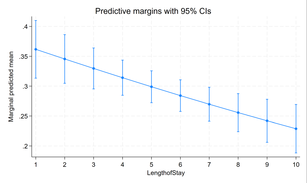
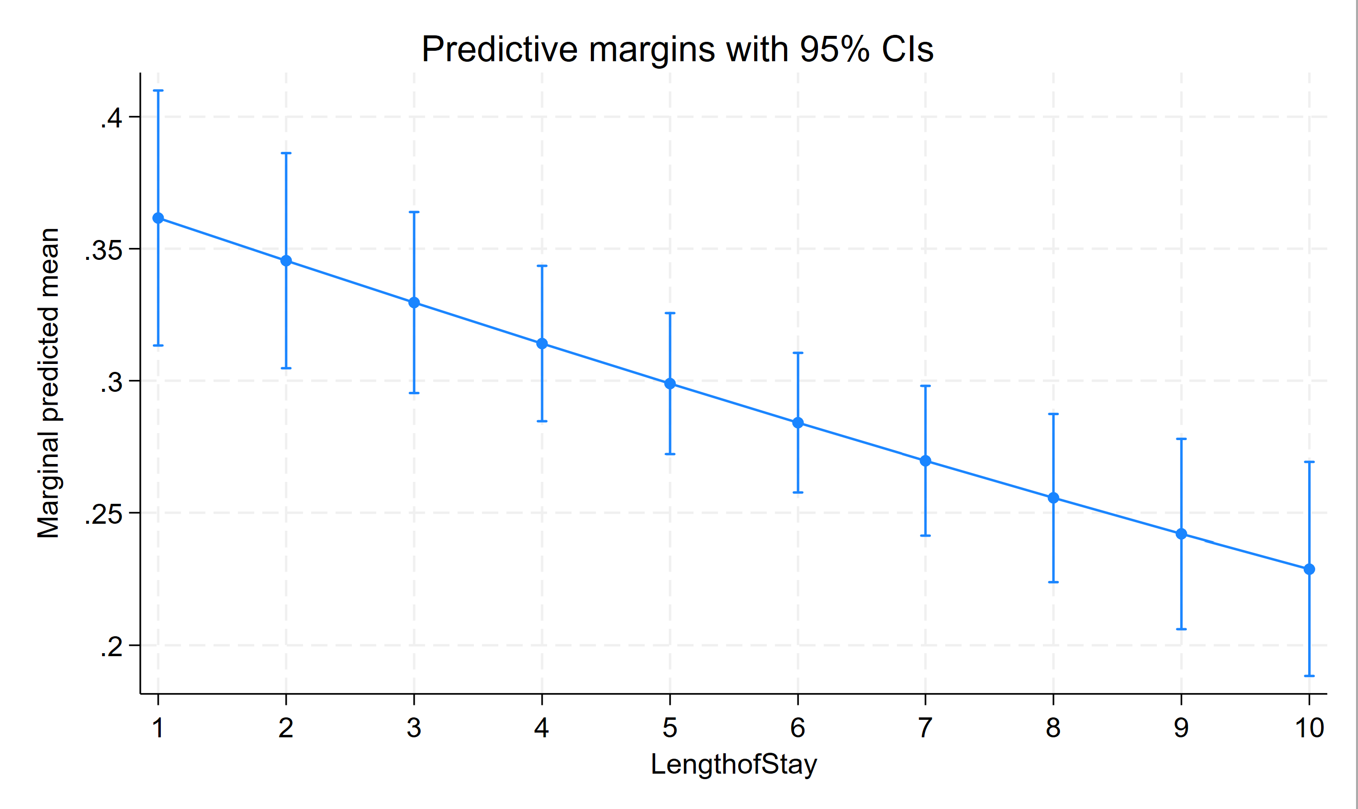
margins, at(lengthofstay=(1(1)10))
Predictive margins Number of obs = 8,525
Model VCE: OIM
Expression: Marginal predicted mean, predict()
1._at: lengthofstay = 1
2._at: lengthofstay = 2
3._at: lengthofstay = 3
4._at: lengthofstay = 4
5._at: lengthofstay = 5
6._at: lengthofstay = 6
7._at: lengthofstay = 7
8._at: lengthofstay = 8
9._at: lengthofstay = 9
10._at: lengthofstay = 10
------------------------------------------------------------------------------
| Delta-method
| Margin std. err. z P>|z| [95% conf. interval]
-------------+----------------------------------------------------------------
_at |
1 | .3616372 .0246409 14.68 0.000 .313342 .4099324
2 | .3454716 .0207823 16.62 0.000 .3047391 .3862042
3 | .3296149 .0174897 18.85 0.000 .2953357 .363894
4 | .3140897 .0150098 20.93 0.000 .284671 .3435084
5 | .2989158 .0136251 21.94 0.000 .2722111 .3256205
6 | .2841097 .0134924 21.06 0.000 .2576651 .3105543
7 | .2696851 .0144703 18.64 0.000 .2413238 .2980465
8 | .2556538 .0162025 15.78 0.000 .2238975 .28741
9 | .2420253 .0183395 13.20 0.000 .2060805 .27797
10 | .2288078 .0206373 11.09 0.000 .1883595 .2692562
------------------------------------------------------------------------------
marginsplot
Three level mixed effects logistic regression
We have looked at a two level logistic model with a random intercept in depth. This is the simplest mixed effects logistic model possible. Now we are going to briefly look at how you can add a third level and random slope effects as well as random intercepts. Below we estimate a three level logistic model with a random intercept for doctors and a random intercept for hospitals. In this examples, doctors are nested within hospitals, meaning that each doctor belongs to one and only one hospital. The alternative case is sometimes called “cross classified” meaning that a doctor may belong to multiple hospitals, such as if some of the doctor’s patients are from hospital A and others from hospital B. Note that this model takes several minutes to run on our machines.
melogit remission age lengthofstay i.familyhx il6 crp i.cancerstage experience || hid: || did:

Fitting fixed-effects model:

Iteration 0:  Log likelihood = -4839.6626
Iteration 1:  Log likelihood = -4827.6553
Iteration 2:  Log likelihood = -4827.5884
Iteration 3:  Log likelihood = -4827.5883

Refining starting values:

Grid node 0:  Log likelihood = -3705.8498

Fitting full model:

Iteration 0:  Log likelihood = -3705.8498  (not concave)
Iteration 1:  Log likelihood = -3701.7405
Iteration 2:  Log likelihood = -3623.3211
Iteration 3:  Log likelihood = -3581.4754
Iteration 4:  Log likelihood = -3580.5544
Iteration 5:  Log likelihood =  -3580.546
Iteration 6:  Log likelihood = -3580.5459

Mixed-effects logistic regression               Number of obs     =      8,525

        Grouping information
        -------------------------------------------------------------
                        |     No. of       Observations per group
         Group variable |     groups    Minimum    Average    Maximum
        ----------------+--------------------------------------------
                    hid |         35        134      243.6        377
                    did |        407          2       20.9         40
        -------------------------------------------------------------

Integration method: mvaghermite                 Integration pts.  =          7

                                                Wald chi2(9)      =     534.44
Log likelihood = -3580.5459                     Prob > chi2       =     0.0000
------------------------------------------------------------------------------
   remission | Coefficient  Std. err.      z    P>|z|     [95% conf. interval]
-------------+----------------------------------------------------------------
         age |  -.0160927    .006067    -2.65   0.008    -.0279837   -.0042017
lengthofstay |  -.0419374   .0364578    -1.15   0.250    -.1133933    .0295185
             |
    familyhx |
        yes  |  -1.309204   .0955226   -13.71   0.000    -1.496425   -1.121983
         il6 |  -.0585677   .0117376    -4.99   0.000    -.0815729   -.0355625
         crp |  -.0232083   .0103834    -2.24   0.025    -.0435593   -.0028573
             |
 cancerstage |
         II  |  -.3218881   .0785581    -4.10   0.000     -.475859   -.1679171
        III  |  -.8635725   .1027077    -8.41   0.000    -1.064876   -.6622691
         IV  |  -2.162947   .1657863   -13.05   0.000    -2.487882   -1.838012
             |
  experience |   .1265195   .0272381     4.64   0.000     .0731339    .1799052
       _cons |  -1.630078   .5807573    -2.81   0.005    -2.768342   -.4918149
-------------+----------------------------------------------------------------
hid          |
   var(_cons)|   .2700061   .1621785                      .0831958    .8762859
-------------+----------------------------------------------------------------
hid>did      |
   var(_cons)|   4.026091   .4284014                      3.268214    4.959716
------------------------------------------------------------------------------
LR test vs. logistic model: chi2(2) = 2494.08             Prob > chi2 = 0.0000

Note: LR test is conservative and provided only for reference.
We can easily add random slopes to the model as well, and allow them to vary at any level. We are just going to add a random slope for lengthofstay that varies between doctors. If estimation problems are encountered, the meqrlogit command can be used.
meqrlogit remission age lengthofstay i.familyhx il6 crp i.cancerstage experience || hid: || did: lengthofstay

Refining starting values:

Iteration 0:  Log likelihood = -3753.4588  (not concave)
Iteration 1:  Log likelihood = -3594.9502  (not concave)
Iteration 2:  Log likelihood = -3558.0874

Performing gradient-based optimization:

Iteration 0:  Log likelihood = -3558.0874
Iteration 1:  Log likelihood = -3553.7133
Iteration 2:  Log likelihood =  -3553.479
Iteration 3:  Log likelihood = -3553.4678
Iteration 4:  Log likelihood = -3553.4677

Mixed-effects logistic regression               Number of obs     =      8,525

----------------------------------------------------------------------------
                |     No. of       Observations per group       Integration
 Group variable |     groups    Minimum    Average    Maximum      points
----------------+-----------------------------------------------------------
            hid |         35        134      243.6        377           7
            did |        407          2       20.9         40           7
----------------------------------------------------------------------------

                                                Wald chi2(9)      =     571.44
Log likelihood = -3553.4677                     Prob > chi2       =     0.0000

------------------------------------------------------------------------------
   remission | Coefficient  Std. err.      z    P>|z|     [95% conf. interval]
-------------+----------------------------------------------------------------
         age |  -.0154721   .0060991    -2.54   0.011    -.0274262    -.003518
lengthofstay |   -.186377   .0455136    -4.09   0.000    -.2755821   -.0971719
             |
    familyhx |
        yes  |  -1.351274   .0971779   -13.91   0.000    -1.541739   -1.160809
         il6 |  -.0591022   .0117973    -5.01   0.000    -.0822244   -.0359799
         crp |  -.0215015   .0104316    -2.06   0.039    -.0419472   -.0010559
             |
 cancerstage |
         II  |  -.2981576   .0784563    -3.80   0.000    -.4519291   -.1443862
        III  |  -.8702162   .1040937    -8.36   0.000    -1.074236   -.6661962
         IV  |  -2.303456   .1723607   -13.36   0.000    -2.641277   -1.965635
             |
  experience |    .106476    .024752     4.30   0.000     .0579629    .1549891
       _cons |  -.5892488   .5665096    -1.04   0.298    -1.699587    .5210895
------------------------------------------------------------------------------

------------------------------------------------------------------------------
  Random-effects parameters  |   Estimate   Std. err.     [95% conf. interval]
-----------------------------+------------------------------------------------
hid: Identity                |
                  var(_cons) |    .544376   .2124416      .2533491    1.169711
-----------------------------+------------------------------------------------
did: Independent             |
               var(length~y) |   .1374912    .022129      .1002941    .1884841
                  var(_cons) |   .2202521   .4743155      .0032348    14.99659
------------------------------------------------------------------------------
LR test vs. logistic model: chi2(3) = 2548.24             Prob > chi2 = 0.0000

Note: LR test is conservative and provided only for reference.
Things to consider
- Sample size: Often the limiting factor is the sample size at the highest unit of analysis. For example, having 500 patients from each of ten doctors would give you a reasonable total number of observations, but not enough to get stable estimates of doctor effects nor of the doctor-to-doctor variation. 10 patients from each of 500 doctors (leading to the same total number of observations) would be preferable.
- Parameter estimation: Because there are not closed form solutions for GLMMs, you must use some approximation. Three are fairly common.
- Quasi-likelihood approaches use a Taylor series expansion to approximate the likelihood. Thus parameters are estimated to maximize the quasi-likelihood. That is, they are not true maximum likelihood estimates. A Taylor series uses a finite set of differentiations of a function to approximate the function, and power rule integration can be performed with Taylor series. With each additional term used, the approximation error decreases (at the limit, the Taylor series will equal the function), but the complexity of the Taylor polynomial also increases. Early quasi-likelihood methods tended to use a first order expansion, more recently a second order expansion is more common. In general, quasi-likelihood approaches are the fastest (although they can still be quite complex), which makes them useful for exploratory purposes and for large datasets. Because of the bias associated with them, quasi-likelihoods are not preferred for final models or statistical inference.
- The true likelihood can also be approximated using numerical integration. Quadrature methods are common, and perhaps most common among these use the Gaussian quadrature rule, frequently with the Gauss-Hermite weighting function. It is also common to incorporate adaptive algorithms that adaptively vary the step size near points with high error. The accuracy increases as the number of integration points increases. Using a single integration point is equivalent to the so-called Laplace approximation. Each additional integration point will increase the number of computations and thus the speed to convergence, although it increases the accuracy. Adaptive Gauss-Hermite quadrature might sound very appealing and is in many ways. However, the number of function evaluations required grows exponentially as the number of dimensions increases. A random intercept is one dimension, adding a random slope would be two. For three level models with random intercepts and slopes, it is easy to create problems that are intractable with Gaussian quadrature. Consequently, it is a useful method when a high degree of accuracy is desired but performs poorly in high dimensional spaces, for large datasets, or if speed is a concern.
- A final set of methods particularly useful for multidimensional integrals are Monte Carlo methods including the famous Metropolis-Hastings algorithm and Gibbs sampling which are types of Markov chain Monte Carlo (MCMC) algorithms. Although Monte Carlo integration can be used in classical statistics, it is more common to see this approach used in Bayesian statistics.
- Complete or quasi-complete separation: Complete separation means that the outcome variable separate a predictor variable completely, leading perfect prediction by the predictor variable. Particularly if the outcome is skewed, there can also be problems with the random effects. For example, if one doctor only had a few patients and all of them either were in remission or were not, there will be no variability within that doctor.
See also
References
- Agresti, A. (2013). Categorical Data Analysis (3rd Ed.), Hoboken, New Jersey: John Wiley & Sons.