Version info: Code for this page was tested in Stata 12.
Robust regression is an alternative to least squares regression when data is contaminated with outliers or influential observations and it can also be used for the purpose of detecting influential observations.
Please note: The purpose of this page is to show how to use various data analysis commands. It does not cover all aspects of the research process which researchers are expected to do. In particular, it does not cover data cleaning and checking, verification of assumptions, model diagnostics or potential follow-up analyses.
Introduction
Let’s begin our discussion on robust regression with some terms in linear regression.
Residual: The difference between the predicted value (based on the regression equation) and the actual, observed value.
Outlier: In linear regression, an outlier is an observation with large residual. In other words, it is an observation whose dependent-variable value is unusual given its value on the predictor variables. An outlier may indicate a sample peculiarity or may indicate a data entry error or other problem.
Leverage: An observation with an extreme value on a predictor variable is a point with high leverage. Leverage is a measure of how far an independent variable deviates from its mean. High leverage points can have a great amount of effect on the estimate of regression coefficients.
Influence: An observation is said to be influential if removing the observation substantially changes the estimate of the regression coefficients. Influence can be thought of as the product of leverage and outlierness.
Cook’s distance (or Cook’s D): A measure that combines the information of leverage and residual of the observation.
Robust regression can be used in any situation in which you would use least squares regression. When fitting a least squares regression, we might find some outliers or high leverage data points. We have decided that these data points are not data entry errors, neither they are from a different population than most of our data. So we have no compelling reason to exclude them from the analysis. Robust regression might be a good strategy since it is a compromise between excluding these points entirely from the analysis and including all the data points and treating all them equally in OLS regression. The idea of robust regression is to weigh the observations differently based on how well behaved these observations are. Roughly speaking, it is a form of weighted and reweighted least squares regression.
Stata’s rreg command implements a version of robust regression. It first runs the OLS regression, gets the Cook’s D for each observation, and then drops any observation with Cook’s distance greater than 1. Then iteration process begins in which weights are calculated based on absolute residuals. The iterating stops when the maximum change between the weights from one iteration to the next is below tolerance. Two types of weights are used. In Huber weighting, observations with small residuals get a weight of 1, the larger the residual, the smaller the weight. With biweighting, all cases with a non-zero residual get down-weighted at least a little. The two different kinds of weight are used because Huber weights can have difficulties with severe outliers, and biweights can have difficulties converging or may yield multiple solutions. Using the Huber weights first helps to minimize problems with the biweights. You can see the iteration history of both types of weights at the top of the robust regression output. Using the Stata defaults, robust regression is about 95% as efficient as OLS (Hamilton, 1991). In short, the most influential points are dropped, and then cases with large absolute residuals are down-weighted.
Description of the data
For our data analysis below, we will use the crime data set. This dataset appears in Statistical Methods for Social Sciences, Third Edition by Alan Agresti and Barbara Finlay (Prentice Hall, 1997). The variables are state id (sid), state name (state), violent crimes per 100,000 people (crime), murders per 1,000,000 (murder), the percent of the population living in metropolitan areas (pctmetro), the percent of the population that is white (pctwhite), percent of population with a high school education or above (pcths), percent of population living under poverty line (poverty), and percent of population that are single parents (single). It has 51 observations. We are going to use poverty and single to predict crime.
use https://stats.idre.ucla.edu/stat/stata/dae/crime, clearsummarize crime poverty single Variable | Obs Mean Std. Dev. Min Max -------------+-------------------------------------------------------- crime | 51 612.8431 441.1003 82 2922 poverty | 51 14.25882 4.584242 8 26.4 single | 51 11.32549 2.121494 8.4 22.1
Robust regression analysis
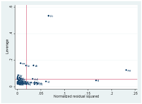
In most cases, we begin by running an OLS regression and doing some diagnostics. We will begin by running an OLS regression. The lvr2plot is used to create a graph showing the leverage versus the squared residuals, and the mlabel option is used to label the points on the graph with the two-letter abbreviation for each state.
regress crime poverty singleSource | SS df MS Number of obs = 51 -------------+------------------------------ F( 2, 48) = 57.96 Model | 6879872.44 2 3439936.22 Prob > F = 0.0000 Residual | 2848602.3 48 59345.8813 R-squared = 0.7072 -------------+------------------------------ Adj R-squared = 0.6950 Total | 9728474.75 50 194569.495 Root MSE = 243.61 ------------------------------------------------------------------------------ crime | Coef. Std. Err. t P>|t| [95% Conf. Interval] -------------+---------------------------------------------------------------- poverty | 6.787359 8.988529 0.76 0.454 -11.28529 24.86001 single | 166.3727 19.42291 8.57 0.000 127.3203 205.425 _cons | -1368.189 187.2052 -7.31 0.000 -1744.59 -991.7874 ------------------------------------------------------------------------------ lvr2plot, mlabel(state)
As we can see, DC, Florida and Mississippi have either high leverage or large residuals. Let’s compute Cook’s D and display the observations that have relatively large values of Cook’s D. To this end, we use the predict command with the cooksd option to create a new variable called d1 containing the values of Cook’s D. Another conventional cut-off point is 4/n, where n is the number of observations in the data set. We will use this criterion to select the values to display.
predict d1, cooksd
clist state crime poverty single d1 if d1>4/51, noobs

    state     crime    poverty     single         d1
       ak       761        9.1       14.3    .125475
       fl      1206       17.8       10.6   .1425891
       ms       434       24.7       14.7   .6138721
       dc      2922       26.4       22.1   2.636252
Since DC has a Cook’s D larger than 1, rreg will assign a missing weight to it so it will be excluded from the robust regression analysis. We probably should drop DC to begin with since it is not even a state. We include it in the analysis just to show that it has large Cook’s D and will be dropped by rreg. Now we will look at the residuals. We will again use the predict command, this time with the rstandard option. We will generate a new variable called absr1, which is the absolute value of the standardized residuals (because the sign of the residual doesn’t matter). The gsort command is used to sort the data by descending order.
predict r1, rstandard
gen absr1 = abs(r1)
gsort -absr1
clist state absr1 in 1/10, noobs

    state      absr1
       ms    3.56299
       fl   2.902663
       dc   2.616447
       vt   1.742409
       mt   1.460884
       me   1.426741
       ak   1.397418
       nj   1.354149
       il   1.338192
       md   1.287087
Now let’s run our robust regression and we will make use of the generate option to have Stata save the final weights to a new variable which we call weight in the data set.
rreg crime poverty single, gen(weight)

   Huber iteration 1:  maximum difference in weights = .66846346
   Huber iteration 2:  maximum difference in weights = .11288069
   Huber iteration 3:  maximum difference in weights = .01810715
Biweight iteration 4:  maximum difference in weights = .29167992
Biweight iteration 5:  maximum difference in weights = .10354281
Biweight iteration 6:  maximum difference in weights = .01421094
Biweight iteration 7:  maximum difference in weights = .0033545

Robust regression                                      Number of obs =      50
                                                       F(  2,    47) =   31.15
                                                       Prob > F      =  0.0000

------------------------------------------------------------------------------
       crime |      Coef.   Std. Err.      t    P>|t|     [95% Conf. Interval]
-------------+----------------------------------------------------------------
     poverty |   10.36971   7.629288     1.36   0.181    -4.978432    25.71786
      single |   142.6339   22.17042     6.43   0.000     98.03276     187.235
       _cons |  -1160.931   224.2564    -5.18   0.000    -1612.076   -709.7849
------------------------------------------------------------------------------
Comparing the OLS regression and robust regression models, we can see that the results are fairly different, especially with respect to the coefficients of single. You will also notice that no R-squared, adjusted R-squared or root MSE from rreg output.
Notice that the number of observations in the robust regression analysis is 50, instead of 51. This is because observation for DC has been dropped since its Cook’s D is greater than 1. We can also see that it is being dropped by looking at the final weight.
clist state weight if state =="dc", noobs

    state      weight
       dc           .
Now let’s look at other observations with relatively small weight.
sort weight
clist sid state weight absr1 d1 in 1/10, noobs

      sid      state      weight      absr1         d1
       25         ms   .02638862    3.56299   .6138721
        9         fl   .11772218   2.902663   .1425891
       46         vt   .59144513   1.742409   .0427155
       26         mt   .66441582   1.460884    .016755
       20         md   .67960728   1.287087   .0356962
       14         il   .69124917   1.338192   .0126569
       21         me   .69766511   1.426741   .0223313
       31         nj   .74574796   1.354149   .0222918
       19         ma   .75392127   1.198541    .016399
        5         ca   .80179038   1.015206   .0123064
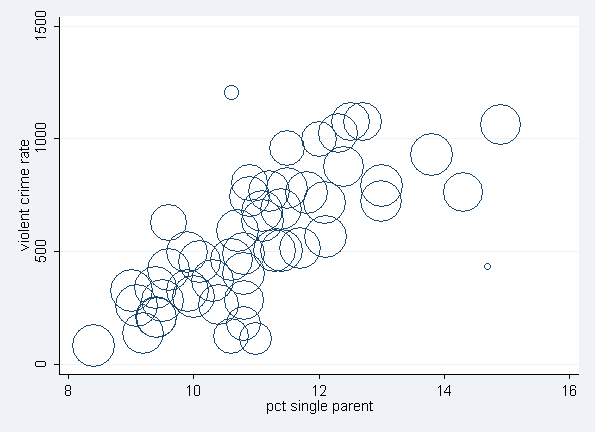
Roughly, as the residual goes down, the weight goes up. In other words, cases with a large residuals tend to be down-weighted, and the values of Cook’s D don’t closely correspond to the weights. This output shows us that the observation for Mississippi will be down-weighted the most. Florida will also be substantially down-weighted. In OLS regression, all cases have a weight of 1. Hence, the more cases in the robust regression that have a weight close to one, the closer the results of the OLS and robust regressions. We can also visualize this relationship by graphing the data points with the weight information as the size of circles.
twoway (scatter crime single [weight=weight], msymbol(oh)) if state !="dc"
Many post-estimation commands are available after running rreg, such as test command and margins command. For example, we can get the predicted values with respect to a set of values of variable single holding poverty at its mean.
margins, at(single=(8(2)22)) vsquish

Predictive margins                                Number of obs   =         50

Expression   : Fitted values, predict()
1._at        : single          =           8
2._at        : single          =          10
3._at        : single          =          12
4._at        : single          =          14
5._at        : single          =          16
6._at        : single          =          18
7._at        : single          =          20
8._at        : single          =          22

------------------------------------------------------------------------------
             |            Delta-method
             |     Margin   Std. Err.      z    P>|z|     [95% Conf. Interval]
-------------+----------------------------------------------------------------
         _at |
          1  |   125.4825   74.88788     1.68   0.094    -21.29505      272.26
          2  |   410.7503   38.20604    10.75   0.000     335.8678    485.6328
          3  |   696.0181    35.2623    19.74   0.000     626.9053    765.1309
          4  |   981.2859   70.42285    13.93   0.000     843.2596    1119.312
          5  |   1266.554   112.2833    11.28   0.000     1046.482    1486.625
          6  |   1551.821   155.5247     9.98   0.000     1246.999    1856.644
          7  |   1837.089     199.25     9.22   0.000     1446.567    2227.612
          8  |   2122.357   243.1982     8.73   0.000     1645.697    2599.017
------------------------------------------------------------------------------
This table shows that as the percent of single parents increases so does the predicted crime rate.
Things to consider
- There are other Stata commands for robust regression written by Stata users. For example, mregress and mmregress by Verardi and Corux implemented more effective M-estimator and MM-estimator. One can get these command via "search mregress" or "search mmregress".
- You might be interested in getting R-squared and other model fit indices, such as AIC or BIC after running rreg. Here is a page that describes a user-written program for obtaining these measures.
- rreg does not address issues of heterogeneity of variance. This problem can be addressed by using the robust option with the regress command.
See also
- Stata 11 Manuals
- Regression with Graphics: A Second Course in Applied Statistics by Lawrence Hamilton
References
- Li, G. 1985. Robust regression. In Exploring Data Tables, Trends, and Shapes, ed. D. C. Hoaglin, F. Mosteller, and J. W. Tukey, Wiley.
- Verardi, V and Croux, C. 2009. Robust regression in Stata. The Stata Journal, Vol 9. No 3
- John Fox, Applied regression analysis, linear models, and related models, Sage publications, Inc, 1997


