The margins command (introduced in Stata 11) is very versatile with numerous options. This page provides information on using the margins command to obtain predicted probabilities.
Let’s get some data and run either a logit model or a probit model. It doesn’t really matter since we can use the same margins commands for either type of model. We will use logit with the binary response variable honors with female as a categorical predictor and read as a continuous predictor. Note that female, which is categorical, is included as a factor variable (i.e. i.female) so that the margins command will treat it as a categorical variable, otherwise, it would be assumed to be continuous.
use https://stats.idre.ucla.edu/stat/data/hsbdemo, clear

logit honors i.female read

Iteration 0:   log likelihood = -115.64441
Iteration 1:   log likelihood = -87.616789
Iteration 2:   log likelihood = -85.457393
Iteration 3:   log likelihood = -85.443724
Iteration 4:   log likelihood =  -85.44372

Logistic regression                               Number of obs   =        200
                                                  LR chi2(2)      =      60.40
                                                  Prob > chi2     =     0.0000
Log likelihood =  -85.44372                       Pseudo R2       =     0.2612

------------------------------------------------------------------------------
      honors |      Coef.   Std. Err.      z    P>|z|     [95% Conf. Interval]
-------------+----------------------------------------------------------------
    1.female |   1.120926   .4081043     2.75   0.006     .3210558    1.920795
        read |   .1443657   .0233338     6.19   0.000     .0986322    .1900991
       _cons |  -9.603364   1.426412    -6.73   0.000    -12.39908   -6.807647
------------------------------------------------------------------------------
We will begin our use of margins by predicting the probabilities for each level of female while holding read at its mean.
margins female, atmeans

Adjusted predictions                              Number of obs   =        200
Model VCE    : OIM

Expression   : Pr(honors), predict()
at           : 0.female        =        .455 (mean)
               1.female        =        .545 (mean)
               read            =       52.23 (mean)

------------------------------------------------------------------------------
             |            Delta-method
             |     Margin   Std. Err.      z    P>|z|     [95% Conf. Interval]
-------------+----------------------------------------------------------------
      female |
          0  |   .1127311   .0350115     3.22   0.001     .0441097    .1813524
          1  |   .2804526   .0509114     5.51   0.000     .1806681    .3802371
------------------------------------------------------------------------------
You can ignore the part of the header that gives the mean for 0.female and 1.female because margins is going to compute the predicted probabilities for each level of female. We do see that read will be held constant at its mean value of 52.23. The values in the column headed Margin are the predicted probabilities for males and females while holding read at its mean.
We also get standard errors z-statistics and p-values testing the difference from zero and a 95% confidence interval for each predicted probability.
Next, we will use margins to get the predicted probabilities for the values of read from 20 to 70 in increments of 10 while holding 1.female at its mean. We will also include the post option so that we can easily get the estimates and their standard errors. We will also include the vsquish option to produce a more compact output.
margins, at(read=(20(10)70)) atmeans vsquish post

Adjusted predictions                              Number of obs   =        200
Model VCE    : OIM

Expression   : Pr(honors), predict()
1._at        : 0.female        =        .455 (mean)
               1.female        =        .545 (mean)
               read            =          20
2._at        : 0.female        =        .455 (mean)
               1.female        =        .545 (mean)
               read            =          30
3._at        : 0.female        =        .455 (mean)
               1.female        =        .545 (mean)
               read            =          40
4._at        : 0.female        =        .455 (mean)
               1.female        =        .545 (mean)
               read            =          50
5._at        : 0.female        =        .455 (mean)
               1.female        =        .545 (mean)
               read            =          60
6._at        : 0.female        =        .455 (mean)
               1.female        =        .545 (mean)
               read            =          70

------------------------------------------------------------------------------
             |            Delta-method
             |     Margin   Std. Err.      z    P>|z|     [95% Conf. Interval]
-------------+----------------------------------------------------------------
         _at |
          1  |   .0022264   .0019625     1.13   0.257    -.0016201    .0060729
          2  |   .0093639   .0061007     1.53   0.125    -.0025934    .0213211
          3  |   .0385002   .0162829     2.36   0.018     .0065864     .070414
          4  |    .145024   .0311995     4.65   0.000      .083874    .2061739
          5  |   .4181148   .0498864     8.38   0.000     .3203393    .5158903
          6  |    .752714   .0670256    11.23   0.000     .6213462    .8840818
------------------------------------------------------------------------------
The variable 1.female is being held at its mean value of 0.545. You can ignore the mean value for 0.female since zero is the reference level of female in our example. The Margin column once again gives the predicted probability. The header above the main part of the table tells us which row is associated with which value of read, Therefore, row 1 is associated with read equal to 20 and row 6 with read equal to 70. It is easy to tell from this table that as the value of read increases the probability of honors being a one is also increasing from a probability of 0.002 to a probability of 0.75.
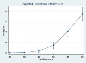
An alternative way to view these results is as a graph that includes the predicted probabilities along with the confidence interval. We will use the marginsplot command for this.
marginsplot

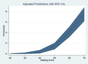
Options can be added to modify the look of the graph.
marginsplot, recast(line) recastci(rarea)

