
Version info: Code for this page was tested in Stata 12.
Zero-truncated negative binomial regression is used to model count data for which the value zero
cannot occur and when there is evidence of over dispersion .
Please Note: The purpose of this page is to show how to use various data analysis commands.
It does not cover all aspects of the research process which researchers are expected to do. In
particular, it does not cover data cleaning and verification, verification of assumptions, model
diagnostics and potential follow-up analyses.
Examples of zero-truncated negative binomial
Example 1.
A study of the length of hospital stay, in days, as a function of age, kind of health insurance and whether
or not the patient died while in the hospital.
Length of hospital stay is recorded as a minimum of at least one day.
Example 2.
A study of the number of journal articles published by tenured faculty as a function of
discipline (fine arts, science, social science, humanities, medical,
etc). To get tenure faculty must publish, i.e., there are no tenured faculty with
zero publications.
Example 3.
A study by the county traffic court on the number of tickets received by teenagers
as predicted by school performance, amount of driver training and gender. Only individuals
who have received at least one citation are in the traffic court files.
Description of the data
Let’s pursue Example 1 from above.
We have a hypothetical data file, ztp.dta with 1,493 observations.
The variable describing length of hospital visit is stay
The variable age gives the age group from 1 to 9 which will be treated as
interval in this example.
The variables hmo and died are binary indicator variables
for HMO insured patients and patients who died while in hospital, respectively. These are the same
data as were used in the ztp example.
Let’s look at the data.
use https://stats.idre.ucla.edu/stat/stata/dae/ztp, clear
summarize stay
Variable | Obs Mean Std. Dev. Min Max
-------------+--------------------------------------------------------
stay | 1493 9.728734 8.132908 1 74
histogram stay, discrete
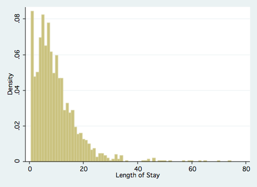 tab1 age hmo died
-> tabulation of age
Age Group | Freq. Percent Cum.
------------+-----------------------------------
1 | 6 0.40 0.40
2 | 60 4.02 4.42
3 | 163 10.92 15.34
4 | 291 19.49 34.83
5 | 317 21.23 56.06
6 | 327 21.90 77.96
7 | 190 12.73 90.69
8 | 93 6.23 96.92
9 | 46 3.08 100.00
------------+-----------------------------------
Total | 1,493 100.00
-> tabulation of hmo
hmo | Freq. Percent Cum.
------------+-----------------------------------
0 | 1,254 83.99 83.99
1 | 239 16.01 100.00
------------+-----------------------------------
Total | 1,493 100.00
-> tabulation of died
died | Freq. Percent Cum.
------------+-----------------------------------
0 | 981 65.71 65.71
1 | 512 34.29 100.00
------------+-----------------------------------
Total | 1,493 100.00
tab1 age hmo died
-> tabulation of age
Age Group | Freq. Percent Cum.
------------+-----------------------------------
1 | 6 0.40 0.40
2 | 60 4.02 4.42
3 | 163 10.92 15.34
4 | 291 19.49 34.83
5 | 317 21.23 56.06
6 | 327 21.90 77.96
7 | 190 12.73 90.69
8 | 93 6.23 96.92
9 | 46 3.08 100.00
------------+-----------------------------------
Total | 1,493 100.00
-> tabulation of hmo
hmo | Freq. Percent Cum.
------------+-----------------------------------
0 | 1,254 83.99 83.99
1 | 239 16.01 100.00
------------+-----------------------------------
Total | 1,493 100.00
-> tabulation of died
died | Freq. Percent Cum.
------------+-----------------------------------
0 | 981 65.71 65.71
1 | 512 34.29 100.00
------------+-----------------------------------
Total | 1,493 100.00
Analysis methods you might consider
Before we show how you can analyze these data with a zero-truncated negative binomial analysis, let’s
consider some other methods that you might use.
- Zero-truncated Negative Binomial Regression – The focus of this web page.
- Zero-truncated Poisson Regression – Useful if there is no overdispersion in the
zero truncated variable. See the Data Analysis Example for ztp. - Negative Binomial Regression – Ordinary negative binomial regression will have difficulty
with zero-truncated data. It will try to predict zero counts even though there are
no zero values. - Poisson Regression – The same concerns as for negative binomial regression, namely,
ordinary poisson regression will have difficulty with
zero-truncated data. It will try to predict zero counts even though there are
no zero values. - OLS Regression – You could try to analyze these data using OLS regression. However, count
data are highly non-normal and are not well estimated by OLS regression.
Zero-truncated negative binomial regression
The tnbreg command will analyze models that are left truncated on any
value not just zero. The ztnb command previously was used for
zero-truncated negative binomial regression, but is no longer supported in
Stata12 and has been superseded by tnbreg.
tnbreg stay age i.hmo i.died, ll(0)

Fitting truncated Poisson model:

Iteration 0:   log likelihood = -6908.7992
Iteration 1:   log likelihood = -6908.7991

Fitting constant-only model:

Iteration 0:   log likelihood =  -4817.852
Iteration 1:   log likelihood = -4778.7604
Iteration 2:   log likelihood = -4770.8734
Iteration 3:   log likelihood =  -4770.848
Iteration 4:   log likelihood =  -4770.848

Fitting full model:

Iteration 0:   log likelihood = -4755.5912
Iteration 1:   log likelihood = -4755.2798
Iteration 2:   log likelihood = -4755.2796

Truncated negative binomial regression            Number of obs   =       1493
Truncation point: 0                               LR chi2(3)      =      31.14
Dispersion     = mean                             Prob > chi2     =     0.0000
Log likelihood = -4755.2796                       Pseudo R2       =     0.0033

------------------------------------------------------------------------------
        stay |      Coef.   Std. Err.      z    P>|z|     [95% Conf. Interval]
-------------+----------------------------------------------------------------
         age |  -.0156929    .013107    -1.20   0.231    -.0413822    .0099964
       1.hmo |  -.1470576   .0592161    -2.48   0.013     -.263119   -.0309962
      1.died |  -.2177714   .0461605    -4.72   0.000    -.3082442   -.1272985
       _cons |   2.408328    .071982    33.46   0.000     2.267245     2.54941
-------------+----------------------------------------------------------------
    /lnalpha |  -.5686389   .0551506                     -.6767321   -.4605457
-------------+----------------------------------------------------------------
       alpha |   .5662957   .0312316                      .5082753    .6309393
------------------------------------------------------------------------------
Likelihood-ratio test of alpha=0:  chibar2(01) = 4307.04 Prob>=chibar2 = 0.000
The output looks very much like the output from an OLS regression:
- It begins with
the iteration log giving the values of the log likelihoods starting
with a model that has no predictors. - The last value in the log (-4755.2796) is the final value
of the log likelihood for the full model and is repeated below. - Next comes the header information. On the right-hand side the number of
observations used (1493) is given along with the likelihood ratio chi-squared with three degrees of
freedom for the full model, followed by the p-value for the chi-square.
The model, as a whole, is statistically significant. - The header also includes
a pseudo-R2, which is very low in this example (0.0033). - Below the header you will find the zero-truncated negative binomial coefficients for each of the variables
along with standard errors, z-scores, p-values and 95% confidence intervals for each
coefficient. - The output also includes an ancillary parameter /lnalpha which is the natural log of the over dispersion
parameter. - Below that, is the the overdispersion parameter alpha along with its standard
error and 95% confidence interval. - Finally, the last line of output is the likelihood-ratio chi-square test that alpha is equal to zero
along with its p-value.
Looking through the results we see the following:
- The value of the coefficient for age, -.0156929, suggests that the log count of
stay decreases by .0156929 for each unit increase in age group. This coefficient is not statistically
significant. - The coefficient for hmo, -.1470576, is significant and indicates that the log count of
stay for HMO patient is .1470576 less than for non-HMO patients. - The log count of stay for patients that died while in the hospital was .2177714 less than
those patients that did not die. - The value of the constant (_cons), 2.408328 is log count of the stay when
all of the predictors equal zero. - The estimate for alpha is .5662957. For comparison, a model
with an alpha
of zero is equivalent to a zero-truncated poisson model. The likelihood-ratio chi-square test that
alpha equals zero is 4307.07 with
one degree of freedom. This is significant result indicates that the negative binomial
model is a better choice than a poisson model.
We can also use the margins command to help understand our model. We will first
compute the expected counts for the categorical variable hmo while holding the continuous
variables age and died at their mean values using the atmeans option.
Please note that the unit for stay is days and not log days for the
margins command.
margins hmo, atmeans

Adjusted predictions                              Number of obs   =       1493
Model VCE    : OIM

Expression   : Predicted number of events, predict()
at           : age             =    5.233758 (mean)
               0.hmo           =    .8399196 (mean)
               1.hmo           =    .1600804 (mean)
               0.died          =    .6570663 (mean)
               1.died          =    .3429337 (mean)

------------------------------------------------------------------------------
             |            Delta-method
             |     Margin   Std. Err.      z    P>|z|     [95% Conf. Interval]
-------------+----------------------------------------------------------------
         hmo |
          0  |   9.502109   .2258589    42.07   0.000     9.059433    9.944784
          1  |   8.202641   .4478629    18.32   0.000     7.324845    9.080436
------------------------------------------------------------------------------
The expected stay for non-HMO patients was 9.502, days while it was 8.203 days for HMO patients.
Using the dydx option computes the difference in expected counts between HMO and non-HMO
patients while still holding the other variables at their mean value.
margins, dydx(hmo) atmeans

Conditional marginal effects                      Number of obs   =       1493
Model VCE    : OIM

Expression   : Predicted number of events, predict()
dy/dx w.r.t. : 1.hmo
at           : age             =    5.233758 (mean)
               0.hmo           =    .8399196 (mean)
               1.hmo           =    .1600804 (mean)
               0.died          =    .6570663 (mean)
               1.died          =    .3429337 (mean)

------------------------------------------------------------------------------
             |            Delta-method
             |      dy/dx   Std. Err.      z    P>|z|     [95% Conf. Interval]
-------------+----------------------------------------------------------------
       1.hmo |  -1.299468   .4985062    -2.61   0.009    -2.276522   -.3224139
------------------------------------------------------------------------------
Note: dy/dx for factor levels is the discrete change from the base level.
As shown above, HMO patients spend 1.299 days less in the hospital than non-HMO patients when the
other variables are held at their mean levels.
One last margins command will give the expected counts for values of age variable from one
through nine while averaging across the two levels of hmo and died. We will
show these results even though age was not statistically significant.
margins, at(age=(1(1)9)) vsquish

Predictive margins                                Number of obs   =       1493
Model VCE    : OIM

Expression   : Predicted number of events, predict()
1._at        : age             =           1
2._at        : age             =           2
3._at        : age             =           3
4._at        : age             =           4
5._at        : age             =           5
6._at        : age             =           6
7._at        : age             =           7
8._at        : age             =           8
9._at        : age             =           9

------------------------------------------------------------------------------
             |            Delta-method
             |     Margin   Std. Err.      z    P>|z|     [95% Conf. Interval]
-------------+----------------------------------------------------------------
         _at |
          1  |   9.984497   .5918896    16.87   0.000     8.824414    11.14458
          2  |   9.829034   .4654886    21.12   0.000     8.916693    10.74138
          3  |   9.675992   .3508834    27.58   0.000     8.988273    10.36371
          4  |   9.525333   .2575035    36.99   0.000     9.020636    10.03003
          5  |    9.37702   .2076088    45.17   0.000     8.970114    9.783926
          6  |   9.231016   .2248183    41.06   0.000      8.79038    9.671652
          7  |   9.087286   .2930141    31.01   0.000     8.512989    9.661583
          8  |   8.945793    .382671    23.38   0.000     8.195772    9.695815
          9  |   8.806504   .4794145    18.37   0.000     7.866868    9.746139
------------------------------------------------------------------------------
A number of model fit indicators are available using the estat ic
command.
estat ic


-----------------------------------------------------------------------------
       Model |    Obs    ll(null)   ll(model)     df          AIC         BIC
-------------+---------------------------------------------------------------
           . |   1493   -4770.848    -4755.28      5     9520.559    9547.102
-----------------------------------------------------------------------------
               Note:  N=Obs used in calculating BIC; see [R] BIC note
Things to consider
- Count data often use an exposure variable to indicate the number of times the event
could have happened. You can incorporate exposure into your model by using the exposure()
option. - It is not recommended that zero-truncated negative binomial models be applied to
small samples. What constitutes a small sample does not seem to be clearly defined
in the literature. - Pseudo-R-squared values differ from OLS R-squareds, please see
FAQ: What are
pseudo R-squareds? for a discussion on this issue.
See Also
- Related Stata Commands
- ztp — zero-truncated poisson regression.
References
- Cameron, A. Colin and Trivedi, P.K. (2009). Microeconometrics using stata. College Station, TX: Stata
Press. - Cameron, A. Colin and Trivedi, P.K. (1998). Regression analysis of
count data. Cambridge, UK: Cambridge University Press. - Hilbe, J. M. (2007). Negative binomial regression. Cambridge, UK: Cambridge
University Press. - Long, J. Scott, & Freese, Jeremy (2006). Regression Models for Categorical Dependent Variables
Using Stata (Second Edition). College Station, TX: Stata Press. - Long, J. Scott (1997). Regression Models for Categorical and Limited Dependent Variables.
Thousand Oaks, CA: Sage Publications.