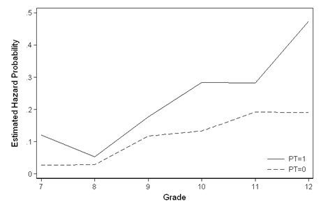
Table 11.1, page 360 and Figure 11.1, page 359.
Note: The noadjust option suppresses the actuarial adjustment.
use https://stats.idre.ucla.edu/stat/stata/examples/alda/data/firstsex, clear
stset time, failure(event)
sts generate s = s, by(pt)
sts generate h = h, by(pt)
sort time
graph twoway (line h time if pt == 1) (line h time if pt == 0), ///
legend(pos(5) ring(0) lab(1 "PT=1") lab(2 "PT=0")) ///
xtitle("Grade") ytitle("Estimated Hazard Probability")
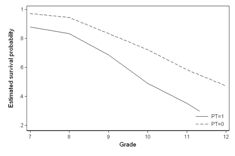
 graph twoway (line s time if pt == 1, sort connect(l)) (line s time if pt == 0, sort connect(l)), ///
legend(pos(5) ring(0) lab(1 "PT=1") lab(2 "PT=0")) ///
xtitle("Grade") ytitle("Estimated survival probability")
graph twoway (line s time if pt == 1, sort connect(l)) (line s time if pt == 0, sort connect(l)), ///
legend(pos(5) ring(0) lab(1 "PT=1") lab(2 "PT=0")) ///
xtitle("Grade") ytitle("Estimated survival probability")
 generate event = ~censor
ltable time event, noadjust survival hazard by(pt)
Beg. Std.
Interval Total Deaths Lost Survival Error [95% Conf. Int.]
-------------------------------------------------------------------------------
pt = 0
7 8 72 2 0 0.9722 0.0194 0.8935 0.9930
8 9 70 2 0 0.9444 0.0270 0.8587 0.9788
9 10 68 8 0 0.8333 0.0439 0.7252 0.9017
10 11 60 8 0 0.7222 0.0528 0.6033 0.8110
11 12 52 10 0 0.5833 0.0581 0.4610 0.6871
12 13 42 8 34 0.4722 0.0588 0.3538 0.5817
pt = 1
7 8 108 13 0 0.8796 0.0313 0.8017 0.9283
8 9 95 5 0 0.8333 0.0359 0.7486 0.8915
9 10 90 16 0 0.6852 0.0447 0.5885 0.7637
10 11 74 21 0 0.4907 0.0481 0.3936 0.5807
11 12 53 15 0 0.3519 0.0460 0.2633 0.4415
12 13 38 18 20 0.1852 0.0374 0.1186 0.2635
-------------------------------------------------------------------------------
Beg. Cum. Std. Std.
Interval Total Failure Error Hazard Error [95% Conf. Int.]
-------------------------------------------------------------------------------
pt 0
7 8 72 0.0278 0.0194 0.0278 0.0196 0.0034 0.0774
8 9 70 0.0556 0.0270 0.0286 0.0202 0.0035 0.0796
9 10 68 0.1667 0.0439 0.1176 0.0416 0.0508 0.2121
10 11 60 0.2778 0.0528 0.1333 0.0471 0.0576 0.2404
11 12 52 0.4167 0.0581 0.1923 0.0608 0.0922 0.3286
12 13 42 0.5278 0.0588 0.1905 0.0673 0.0822 0.3434
pt 1
7 8 108 0.1204 0.0313 0.1204 0.0334 0.0641 0.1941
8 9 95 0.1667 0.0359 0.0526 0.0235 0.0171 0.1078
9 10 90 0.3148 0.0447 0.1778 0.0444 0.1016 0.2749
10 11 74 0.5093 0.0481 0.2838 0.0619 0.1757 0.4174
11 12 53 0.6481 0.0460 0.2830 0.0731 0.1584 0.4432
12 13 38 0.8148 0.0374 0.4737 0.1116 0.2807 0.7163
-------------------------------------------------------------------------------
ltable time event, noadjust survival hazard
Beg. Std.
Interval Total Deaths Lost Survival Error [95% Conf. Int.]
-------------------------------------------------------------------------------
7 8 180 15 0 0.9167 0.0206 0.8656 0.9489
8 9 165 7 0 0.8778 0.0244 0.8203 0.9178
9 10 158 24 0 0.7444 0.0325 0.6741 0.8019
10 11 134 29 0 0.5833 0.0367 0.5078 0.6514
11 12 105 25 0 0.4444 0.0370 0.3709 0.5153
12 13 80 26 54 0.3000 0.0342 0.2348 0.3678
-------------------------------------------------------------------------------
Beg. Cum. Std. Std.
Interval Total Failure Error Hazard Error [95% Conf. Int.]
-------------------------------------------------------------------------------
7 8 180 0.0833 0.0206 0.0833 0.0215 0.0466 0.1305
8 9 165 0.1222 0.0244 0.0424 0.0160 0.0171 0.0791
9 10 158 0.2556 0.0325 0.1519 0.0310 0.0973 0.2184
10 11 134 0.4167 0.0367 0.2164 0.0402 0.1449 0.3020
11 12 105 0.5556 0.0370 0.2381 0.0476 0.1541 0.3401
12 13 80 0.7000 0.0342 0.3250 0.0637 0.2123 0.4613
-------------------------------------------------------------------------------
generate event = ~censor
ltable time event, noadjust survival hazard by(pt)
Beg. Std.
Interval Total Deaths Lost Survival Error [95% Conf. Int.]
-------------------------------------------------------------------------------
pt = 0
7 8 72 2 0 0.9722 0.0194 0.8935 0.9930
8 9 70 2 0 0.9444 0.0270 0.8587 0.9788
9 10 68 8 0 0.8333 0.0439 0.7252 0.9017
10 11 60 8 0 0.7222 0.0528 0.6033 0.8110
11 12 52 10 0 0.5833 0.0581 0.4610 0.6871
12 13 42 8 34 0.4722 0.0588 0.3538 0.5817
pt = 1
7 8 108 13 0 0.8796 0.0313 0.8017 0.9283
8 9 95 5 0 0.8333 0.0359 0.7486 0.8915
9 10 90 16 0 0.6852 0.0447 0.5885 0.7637
10 11 74 21 0 0.4907 0.0481 0.3936 0.5807
11 12 53 15 0 0.3519 0.0460 0.2633 0.4415
12 13 38 18 20 0.1852 0.0374 0.1186 0.2635
-------------------------------------------------------------------------------
Beg. Cum. Std. Std.
Interval Total Failure Error Hazard Error [95% Conf. Int.]
-------------------------------------------------------------------------------
pt 0
7 8 72 0.0278 0.0194 0.0278 0.0196 0.0034 0.0774
8 9 70 0.0556 0.0270 0.0286 0.0202 0.0035 0.0796
9 10 68 0.1667 0.0439 0.1176 0.0416 0.0508 0.2121
10 11 60 0.2778 0.0528 0.1333 0.0471 0.0576 0.2404
11 12 52 0.4167 0.0581 0.1923 0.0608 0.0922 0.3286
12 13 42 0.5278 0.0588 0.1905 0.0673 0.0822 0.3434
pt 1
7 8 108 0.1204 0.0313 0.1204 0.0334 0.0641 0.1941
8 9 95 0.1667 0.0359 0.0526 0.0235 0.0171 0.1078
9 10 90 0.3148 0.0447 0.1778 0.0444 0.1016 0.2749
10 11 74 0.5093 0.0481 0.2838 0.0619 0.1757 0.4174
11 12 53 0.6481 0.0460 0.2830 0.0731 0.1584 0.4432
12 13 38 0.8148 0.0374 0.4737 0.1116 0.2807 0.7163
-------------------------------------------------------------------------------
ltable time event, noadjust survival hazard
Beg. Std.
Interval Total Deaths Lost Survival Error [95% Conf. Int.]
-------------------------------------------------------------------------------
7 8 180 15 0 0.9167 0.0206 0.8656 0.9489
8 9 165 7 0 0.8778 0.0244 0.8203 0.9178
9 10 158 24 0 0.7444 0.0325 0.6741 0.8019
10 11 134 29 0 0.5833 0.0367 0.5078 0.6514
11 12 105 25 0 0.4444 0.0370 0.3709 0.5153
12 13 80 26 54 0.3000 0.0342 0.2348 0.3678
-------------------------------------------------------------------------------
Beg. Cum. Std. Std.
Interval Total Failure Error Hazard Error [95% Conf. Int.]
-------------------------------------------------------------------------------
7 8 180 0.0833 0.0206 0.0833 0.0215 0.0466 0.1305
8 9 165 0.1222 0.0244 0.0424 0.0160 0.0171 0.0791
9 10 158 0.2556 0.0325 0.1519 0.0310 0.0973 0.2184
10 11 134 0.4167 0.0367 0.2164 0.0402 0.1449 0.3020
11 12 105 0.5556 0.0370 0.2381 0.0476 0.1541 0.3401
12 13 80 0.7000 0.0342 0.3250 0.0637 0.2123 0.4613
-------------------------------------------------------------------------------
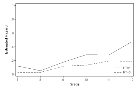
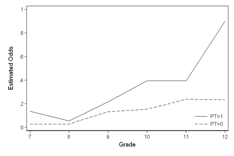
Figure 11.2, page 363.
sort time
gen estodds = h/(1-h)
gen logith = log(h/(1-h))
graph twoway (line h time if pt == 1) (line h time if pt == 0), ///
ylabel(0(.2)1) legend(pos(5) ring(0) lab(1 "PT=1") lab(2 "PT=0")) ///
xtitle("Grade") ytitle("Estimated Hazard")
 graph twoway (line estodds time if pt == 1) (line estodds time if pt == 0), ///
ylabel(0(.2)1) legend(pos(5) ring(0) lab(1 "PT=1") lab(2 "PT=0")) ///
xtitle("Grade") ytitle("Estimated Odds")
graph twoway (line estodds time if pt == 1) (line estodds time if pt == 0), ///
ylabel(0(.2)1) legend(pos(5) ring(0) lab(1 "PT=1") lab(2 "PT=0")) ///
xtitle("Grade") ytitle("Estimated Odds")
 graph twoway (line logith time if pt == 1) (line logith time if pt == 0), ///
legend(pos(5) ring(0) lab(1 "PT=1") lab(2 "PT=0")) ///
xtitle("Grade") ytitle("Estimated logit(hazard)")
graph twoway (line logith time if pt == 1) (line logith time if pt == 0), ///
legend(pos(5) ring(0) lab(1 "PT=1") lab(2 "PT=0")) ///
xtitle("Grade") ytitle("Estimated logit(hazard)")
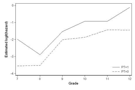
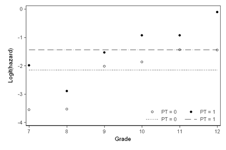
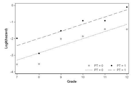
Figure 11.3, page 366.
use https://stats.idre.ucla.edu/stat/stata/examples/alda/data/firstsex_pp, clear
egen c1 = count(id), by(period pt)
egen c2 = count(id), by(period pt event)
generate prob = c2/c1
gen pt0 = log(prob/(1-prob)) if event==1 & pt==0
gen pt1 = log(prob/(1-prob)) if event==1 & pt==1
quietly logit event pt
predict p1
generate lp1 = log(p1/(1-p1))
sort pt period
graph twoway (scatter pt0 period) (scatter pt1 period) ///
(line lp1 period if pt==0) (line lp1 period if pt==1), ///
legend(ring(0) pos(5) col(2) ///
lab(1 "PT = 0") lab(2 "PT = 1") lab(3 "PT = 0") lab(4 "PT = 1")) ///
xtitle("Grade") ytitle("Logit(hazard)")
 quietly logit event period pt
predict p2
generate lp2 = log(p2/(1-p2))
graph twoway (scatter pt0 period) (scatter pt1 period) ///
(line lp2 period if pt==0) (line lp2 period if pt==1), ///
legend(ring(0) pos(5) col(2) ///
lab(1 "PT = 0") lab(2 "PT = 1") lab(3 "PT = 0") lab(4 "PT = 1")) ///
xtitle("Grade") ytitle("Logit(hazard)")
quietly logit event period pt
predict p2
generate lp2 = log(p2/(1-p2))
graph twoway (scatter pt0 period) (scatter pt1 period) ///
(line lp2 period if pt==0) (line lp2 period if pt==1), ///
legend(ring(0) pos(5) col(2) ///
lab(1 "PT = 0") lab(2 "PT = 1") lab(3 "PT = 0") lab(4 "PT = 1")) ///
xtitle("Grade") ytitle("Logit(hazard)")
 quietly logit event d7 d8 d9 d10 d11 d12 pt, nocons
predict p3
generate lp3 = log(p3/(1-p3))
graph twoway (scatter pt0 period) (scatter pt1 period) ///
(line lp3 period if pt==0) (line lp3 period if pt==1), ///
legend(ring(0) pos(5) col(2) ///
lab(1 "PT = 0") lab(2 "PT = 1") lab(3 "PT = 0") lab(4 "PT = 1")) ///
xtitle("Grade") ytitle("Logit(hazard)")
quietly logit event d7 d8 d9 d10 d11 d12 pt, nocons
predict p3
generate lp3 = log(p3/(1-p3))
graph twoway (scatter pt0 period) (scatter pt1 period) ///
(line lp3 period if pt==0) (line lp3 period if pt==1), ///
legend(ring(0) pos(5) col(2) ///
lab(1 "PT = 0") lab(2 "PT = 1") lab(3 "PT = 0") lab(4 "PT = 1")) ///
xtitle("Grade") ytitle("Logit(hazard)")
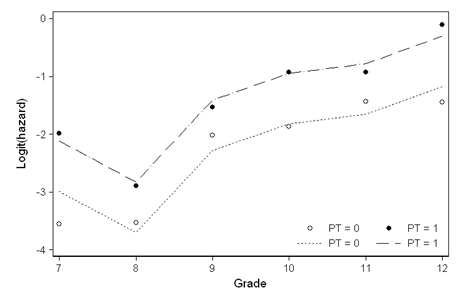
Figure 11.4, page 374.
quietly logit event d7 d8 d9 d10 d11 d12 pt, nocons
predict pA
gen lpA = logit(pA)
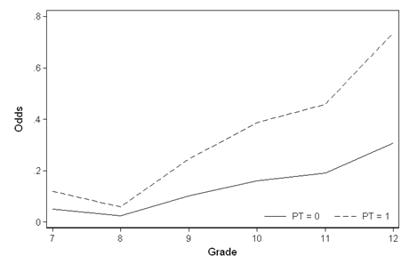
gen estods = exp(logit(pA))
sort period
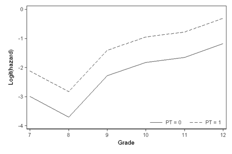
graph twoway (line lpA period if pt==0) (line lpA period if pt==1), ///
legend(ring(0) pos(5) col(2) ///
lab(1 "PT = 0") lab(2 "PT = 1")) ///
xtitle("Grade") ytitle("Logit(hazard)")
 graph twoway (line estods period if pt==0) (line estods period if pt==1), ///
legend(ring(0) pos(5) col(2) ///
lab(1 "PT = 0") lab(2 "PT = 1")) ///
ylabel(0(.2).8) xtitle("Grade") ytitle("Odds")
graph twoway (line estods period if pt==0) (line estods period if pt==1), ///
legend(ring(0) pos(5) col(2) ///
lab(1 "PT = 0") lab(2 "PT = 1")) ///
ylabel(0(.2).8) xtitle("Grade") ytitle("Odds")
 graph twoway (line pA period if pt==0) (line pA period if pt==1), ///
legend(ring(0) pos(5) col(2) ///
lab(1 "PT = 0") lab(2 "PT = 1")) ///
ylabel(0(.1).5) xtitle("Grade") ytitle("Hazard")
graph twoway (line pA period if pt==0) (line pA period if pt==1), ///
legend(ring(0) pos(5) col(2) ///
lab(1 "PT = 0") lab(2 "PT = 1")) ///
ylabel(0(.1).5) xtitle("Grade") ytitle("Hazard")
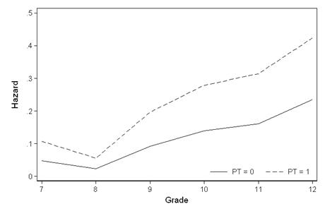
Table 11.3, page 386.
Note: This table makes use of fitstat.ado written by J. Scott Long and Jeremy Freese to obtain the deviance, and information criterion statistics. You can obtain fitstat.ado by typing, search fitstat (see How can I use the search command to search for programs and get additional help? for more information about using search). In order to use fitstat you must first run the model with a constant. We will not display output from the model containing the constant.
Note: The BIC values are different from those in the book. Clearly, they are based on different algorithms. In general, with AIC and BIC, smaller is better.
use https://stats.idre.ucla.edu/stat/stata/examples/alda/data/firstsex_pp, clear

/* Model A */
logit event d7 d8 d9 d10 d11 d12, nocons

Logit estimates                                   Number of obs   =        822
                                                  LR chi2(6)      =          .
Log likelihood = -325.97769                       Prob > chi2     =          .

------------------------------------------------------------------------------
       event |      Coef.   Std. Err.      z    P>|z|     [95% Conf. Interval]
-------------+----------------------------------------------------------------
          d7 |  -2.397895   .2696799    -8.89   0.000    -2.926458   -1.869332
          d8 |  -3.116685   .3862453    -8.07   0.000    -3.873712   -2.359658
          d9 |  -1.719786   .2216514    -7.76   0.000    -2.154215   -1.285357
         d10 |  -1.286665   .2097774    -6.13   0.000    -1.697821   -.8755083
         d11 |  -1.163151   .2291288    -5.08   0.000    -1.612235   -.7140666
         d12 |  -.7308875    .238705    -3.06   0.002    -1.198741   -.2630344
------------------------------------------------------------------------------

quietly logit event d7 d8 d9 d10 d11 d12
fitstat

Measures of Fit for logit of event

Log-Lik Intercept Only:     -352.116     Log-Lik Full Model:         -325.978
D(816):                      651.955     LR(5):                        52.276
                                         Prob > LR:                     0.000
McFadden's R2:                 0.074     McFadden's Adj R2:             0.057
Maximum Likelihood R2:         0.062     Cragg & Uhler's R2:            0.107
McKelvey and Zavoina's R2:     0.159     Efron's R2:                    0.061
Variance of y*:                3.912     Variance of error:             3.290
Count R2:                      0.847     Adj Count R2:                  0.000
AIC:                           0.808     AIC*n:                       663.955
BIC:                       -4824.825     BIC':                        -18.717

/* Model B */
logit event d7 d8 d9 d10 d11 d12 pt, nocons

Logit estimates                                   Number of obs   =        822
                                                  LR chi2(7)      =          .
Log likelihood = -317.33089                       Prob > chi2     =          .

------------------------------------------------------------------------------
       event |      Coef.   Std. Err.      z    P>|z|     [95% Conf. Interval]
-------------+----------------------------------------------------------------
          d7 |  -2.994327   .3175088    -9.43   0.000    -3.616632   -2.372021
          d8 |  -3.700124   .4205614    -8.80   0.000    -4.524409   -2.875839
          d9 |  -2.281124   .2723919    -8.37   0.000    -2.815002   -1.747245
         d10 |  -1.822599   .2584613    -7.05   0.000    -2.329173   -1.316024
         d11 |  -1.654227   .2691057    -6.15   0.000    -2.181665    -1.12679
         d12 |  -1.179057   .2715801    -4.34   0.000    -1.711344   -.6467698
          pt |   .8736184   .2174075     4.02   0.000     .4475076    1.299729
------------------------------------------------------------------------------

quietly logit event d7 d8 d9 d10 d11 d12 pt
fitstat

Measures of Fit for logit of event

Log-Lik Intercept Only:     -352.116     Log-Lik Full Model:         -317.331
D(815):                      634.662     LR(6):                        69.570
                                         Prob > LR:                     0.000
McFadden's R2:                 0.099     McFadden's Adj R2:             0.079
Maximum Likelihood R2:         0.081     Cragg & Uhler's R2:            0.141
McKelvey and Zavoina's R2:     0.202     Efron's R2:                    0.087
Variance of y*:                4.121     Variance of error:             3.290
Count R2:                      0.847     Adj Count R2:                  0.000
AIC:                           0.789     AIC*n:                       648.662
BIC:                       -4835.407     BIC':                        -29.299

test pt   /* wald test */

 ( 1)  pt = 0.0

           chi2(  1) =   16.15
         Prob > chi2 =    0.0000

/* Model C */
logit event d7 d8 d9 d10 d11 d12 pas, nocons

Logit estimates                                   Number of obs   =        822
                                                  LR chi2(7)      =          .
Log likelihood = -318.58429                       Prob > chi2     =          .

------------------------------------------------------------------------------
       event |      Coef.   Std. Err.      z    P>|z|     [95% Conf. Interval]
-------------+----------------------------------------------------------------
          d7 |  -2.464565   .2741086    -8.99   0.000    -3.001808   -1.927322
          d8 |  -3.159096   .3890048    -8.12   0.000    -3.921532   -2.396661
          d9 |  -1.729688   .2244951    -7.70   0.000    -2.169691   -1.289686
         d10 |  -1.285083   .2126567    -6.04   0.000    -1.701882   -.8682836
         d11 |   -1.13596   .2323622    -4.89   0.000    -1.591381   -.6805382
         d12 |  -.6420982   .2428271    -2.64   0.008    -1.118031   -.1661658
         pas |      .4428   .1139575     3.89   0.000     .2194475    .6661525
------------------------------------------------------------------------------

quietly logit event d7 d8 d9 d10 d11 d12 pas
fitstat

Measures of Fit for logit of event

Log-Lik Intercept Only:     -352.116     Log-Lik Full Model:         -318.584
D(815):                      637.169     LR(6):                        67.063
                                         Prob > LR:                     0.000
McFadden's R2:                 0.095     McFadden's Adj R2:             0.075
Maximum Likelihood R2:         0.078     Cragg & Uhler's R2:            0.136
McKelvey and Zavoina's R2:     0.193     Efron's R2:                    0.081
Variance of y*:                4.079     Variance of error:             3.290
Count R2:                      0.850     Adj Count R2:                  0.024
AIC:                           0.792     AIC*n:                       651.169
BIC:                       -4832.900     BIC':                        -26.792

test pas   /* wald test */

 ( 1)  pas = 0.0

           chi2(  1) =   15.10
         Prob > chi2 =    0.0001

/* Model D */
logit event d7 d8 d9 d10 d11 d12 pt pas, nocons


Logit estimates                                   Number of obs   =        822
                                                  LR chi2(8)      =          .
Log likelihood = -314.57348                       Prob > chi2     =          .

------------------------------------------------------------------------------
       event |      Coef.   Std. Err.      z    P>|z|     [95% Conf. Interval]
-------------+----------------------------------------------------------------
          d7 |  -2.893237   .3206302    -9.02   0.000     -3.52166   -2.264813
          d8 |  -3.584759   .4231464    -8.47   0.000    -4.414111   -2.755407
          d9 |  -2.150233    .277458    -7.75   0.000    -2.694041   -1.606426
         d10 |   -1.69318   .2646518    -6.40   0.000    -2.211888   -1.174472
         d11 |  -1.517695   .2757453    -5.50   0.000    -2.058146   -.9772446
         d12 |  -1.009884   .2811314    -3.59   0.000    -1.560891   -.4588762
          pt |   .6605301   .2367272     2.79   0.005     .1965533    1.124507
         pas |   .2963606   .1253783     2.36   0.018     .0506236    .5420976
------------------------------------------------------------------------------

quietly logit event d7 d8 d9 d10 d11 d12 pt pas
fitstat

Measures of Fit for logit of event

Log-Lik Intercept Only:     -352.116     Log-Lik Full Model:         -314.573
D(814):                      629.147     LR(7):                        75.084
                                         Prob > LR:                     0.000
McFadden's R2:                 0.107     McFadden's Adj R2:             0.084
Maximum Likelihood R2:         0.087     Cragg & Uhler's R2:            0.152
McKelvey and Zavoina's R2:     0.214     Efron's R2:                    0.093
Variance of y*:                4.183     Variance of error:             3.290
Count R2:                      0.850     Adj Count R2:                  0.024
AIC:                           0.785     AIC*n:                       645.147
BIC:                       -4834.210     BIC':                        -28.102

test pt   /* wald test */

 ( 1)  pt = 0.0

           chi2(  1) =    7.79
         Prob > chi2 =    0.0053

test pas   /* wald test */

 ( 1)  pas = 0.0

           chi2(  1) =    5.59
         Prob > chi2 =    0.0181
Table 11.4, page 388.
use https://stats.idre.ucla.edu/stat/stata/examples/alda/data/firstsex_pp, clear
quietly logit event d7 d8 d9 d10 d11 d12, nocons
predict p
preserve
collapse (mean) p, by(period)
gen paramest = logit(p)
gen odds = exp(paramest)

clist period paramest odds p

        period   paramest       odds          p
  1.         7  -2.397895   .0909091   .0833333
  2.         8  -3.116685   .0443038   .0424242
  3.         9  -1.719786   .1791045   .1518987
  4.        10  -1.286664   .2761905   .2164179
  5.        11  -1.163151      .3125   .2380952
  6.        12  -.7308876   .4814814       .325
Table 11.5, page 392.
use https://stats.idre.ucla.edu/stat/stata/examples/alda/data/firstsex_pp, clear
quietly logit event d7 d8 d9 d10 d11 d12 pt, nocons
predict p
collapse (mean) p, by(period pt)
reshape wide p, i(period) j(pt)
gen logith0 = logit(p0)
gen logith1 = logit(p1)
gen surv_0 = 1
replace surv_0 = (1 - p0)*surv_0 if period == 7
replace surv_0 = (1 - p0)*surv_0[_n-1] if period > 7
gen surv_1 = 1
replace surv_1 = (1 - p1)*surv_1 if period == 7
replace surv_1 = (1 - p1)*surv_1[_n-1] if period > 7

clist period logith0 logith1 p0 p1 surv_0 surv_1

        period    logith0    logith1         p0         p1     surv_0     surv_1
  1.         7  -2.994327  -2.120708   .0476828   .1071003   .9523172   .8928997
  2.         8  -3.700124  -2.826506   .0241241   .0559086   .9293434    .842979
  3.         9  -2.281124  -1.407505   .0926984   .1966279   .8431947   .6772258
  4.        10  -1.822598    -.94898   .1391224     .27909   .7258875   .4882188
  5.        11  -1.654227  -.7806088   .1605384   .3141887   .6093546    .334826
  6.        12  -1.179057  -.3054385   .2352218   .4242285   .4660211   .1927833
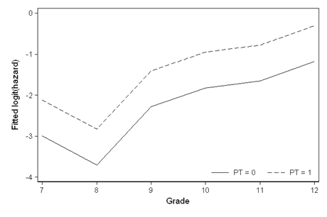
Figure 11.6, page 393.
graph twoway (line logith0 period) (line logith1 period), ///
legend(ring(0) pos(5) col(2) ///
lab(1 "PT = 0") lab(2 "PT = 1")) ///
xtitle("Grade") ytitle("Fitted logit(hazard)")
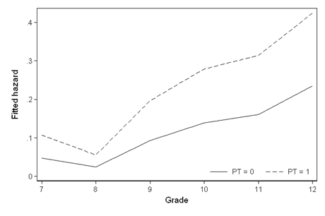
 graph twoway (line p0 period) (line p1 period), ///
legend(ring(0) pos(5) col(2) ///
lab(1 "PT = 0") lab(2 "PT = 1")) ///
xtitle("Grade") ytitle("Fitted hazard")
graph twoway (line p0 period) (line p1 period), ///
legend(ring(0) pos(5) col(2) ///
lab(1 "PT = 0") lab(2 "PT = 1")) ///
xtitle("Grade") ytitle("Fitted hazard")
 graph twoway (line surv_0 period) (line surv_1 period), ///
legend(ring(0) pos(5) col(2) ///
lab(1 "PT = 0") lab(2 "PT = 1")) ///
xtitle("Grade") ytitle("Fitted Survival Probability")
graph twoway (line surv_0 period) (line surv_1 period), ///
legend(ring(0) pos(5) col(2) ///
lab(1 "PT = 0") lab(2 "PT = 1")) ///
xtitle("Grade") ytitle("Fitted Survival Probability")
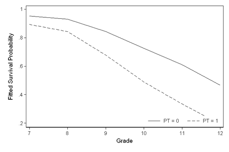
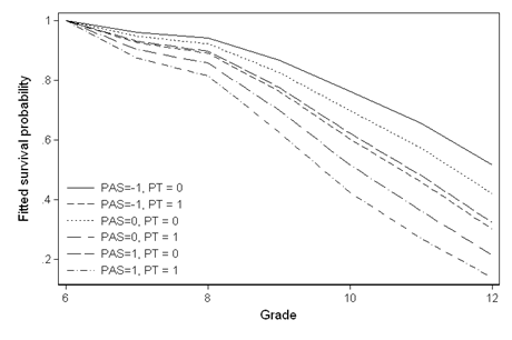
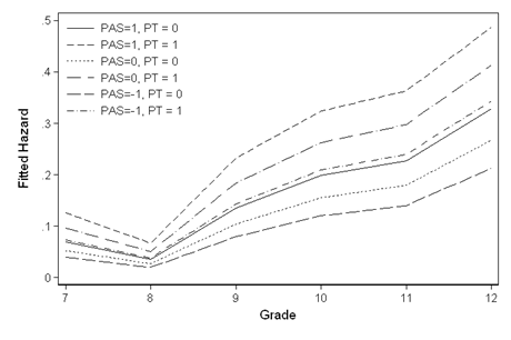
Figure 11.7, page 395.
use https://stats.idre.ucla.edu/stat/stata/examples/alda/data/firstsex_pp, clear
logit event d7 d8 d9 d10 d11 d12 pt pas, nocons

gen pas0 = -2.893237*d7 - 3.584759*d8 - 2.150233*d9 - 1.69318*d10 - 1.517695*d11 - 1.009884*d12 + .6605301*pt
gen pas1 = pas0 + .2963606
gen pasneg1 = pas0 - .2963606

collapse (mean) pas0 pas1 pasneg1, by(period pt)

gen pas0_p = exp(pas0)/(1+exp(pas0))
gen pas1_p = exp(pas1)/(1+exp(pas1))
gen pasneg1_p = exp(pasneg1)/(1+exp(pasneg1))

/* top figure */
twoway (line pas1_p period if pt==0)(line pas1_p period if pt==1) ///
 (line pas0_p period if pt==0)(line pas0_p  period if pt==1) ///
 (line pasneg1_p period if pt==0)(line pasneg1_p period if pt==1), ///
 xtitle("Grade") ytitle("Fitted Hazard") legend(ring(0) pos(10) col(1) ///
 lab(1 "PAS=1, PT = 0") lab(2 "PAS=1, PT = 1") lab(3 "PAS=0, PT = 0") ///
 lab(4 "PAS=0, PT = 1") lab(5 "PAS=-1, PT = 0") lab(6 "PAS=-1, PT = 1"))


set obs 14
replace period = 6 if period == .
replace pt = 0 if _n==13
replace pt = 1 if _n==14

gen surv_neg1 = 1
replace surv_neg1 = (1 - pasneg1_p)*surv_neg1 if period == 7
replace surv_neg1 = (1 - pasneg1_p)*surv_neg1[_n-2] if period > 7

gen surv_0 = 1
replace surv_0 = (1 - pas0_p)*surv_0 if period == 7
replace surv_0 = (1 - pas0_p)*surv_0[_n-2] if period > 7

gen surv_1 = 1
replace surv_1 = (1 - pas1_p)*surv_1 if period == 7
replace surv_1 = (1 - pas1_p)*surv_1[_n-2] if period > 7


/* top figure */
sort period
twoway (line surv_neg1 period if pt==0)(line surv_neg1 period if pt==1) ///
 (line surv_0 period if pt==0)(line surv_0 period if pt==1) ///
 (line surv_1 period if pt==0)(line surv_1 period if pt==1), ///
 xtitle("Grade") ytitle("Fitted survival probability") legend(ring(0) pos(7) col(1) ///
 lab(1 "PAS=-1, PT = 0") lab(2 "PAS=-1, PT = 1") lab(3 "PAS=0, PT = 0") ///
 lab(4 "PAS=0, PT = 1") lab(5 "PAS=1, PT = 0") lab(6 "PAS=1, PT = 1"))
set obs 14
replace period = 6 if period == .
replace pt = 0 if _n==13
replace pt = 1 if _n==14
gen surv_neg1 = 1
replace surv_neg1 = (1 - pasneg1_p)*surv_neg1 if period == 7
replace surv_neg1 = (1 - pasneg1_p)*surv_neg1[_n-2] if period > 7
gen surv_0 = 1
replace surv_0 = (1 - pas0_p)*surv_0 if period == 7
replace surv_0 = (1 - pas0_p)*surv_0[_n-2] if period > 7
gen surv_1 = 1
replace surv_1 = (1 - pas1_p)*surv_1 if period == 7
replace surv_1 = (1 - pas1_p)*surv_1[_n-2] if period > 7
/* top figure */
sort period
twoway (line surv_neg1 period if pt==0)(line surv_neg1 period if pt==1) ///
(line surv_0 period if pt==0)(line surv_0 period if pt==1) ///
(line surv_1 period if pt==0)(line surv_1 period if pt==1), ///
xtitle("Grade") ytitle("Fitted survival probability") legend(ring(0) pos(7) col(1) ///
lab(1 "PAS=-1, PT = 0") lab(2 "PAS=-1, PT = 1") lab(3 "PAS=0, PT = 0") ///
lab(4 "PAS=0, PT = 1") lab(5 "PAS=1, PT = 0") lab(6 "PAS=1, PT = 1"))