Figure 2.1, page 18.
use https://stats.idre.ucla.edu/stat/stata/examples/alda/data/tolerance, clear
list

            id      tol11      tol12      tol13      tol14      tol15       male   exposure
  1.         9       2.23       1.79        1.9       2.12       2.66          0       1.54
  2.        45       1.12       1.45       1.45       1.45       1.99          1       1.16
  3.       268       1.45       1.34       1.99       1.79       1.34          1         .9
  4.       314       1.22       1.22       1.55       1.12       1.12          0        .81
  5.       442       1.45       1.99       1.45       1.67        1.9          0       1.13
  6.       514       1.34       1.67       2.23       2.12       2.44          1         .9
  7.       569       1.79        1.9        1.9       1.99       1.99          0       1.99
  8.       624       1.12       1.12       1.22       1.12       1.22          1        .98
  9.       723       1.22       1.34       1.12          1       1.12          0        .81
 10.       918          1          1       1.22       1.99       1.22          0       1.21
 11.       949       1.99       1.55       1.12       1.45       1.55          1        .93
 12.       978       1.22       1.34       2.12       3.46       3.32          1       1.59
 13.      1105       1.34        1.9       1.99        1.9       2.12          1       1.38
 14.      1542       1.22       1.22       1.99       1.79       2.12          0       1.44
 15.      1552          1       1.12       2.23       1.55       1.55          0       1.04
 16.      1653       1.11       1.11       1.34       1.55       2.12          0       1.25

reshape long tol, i(id) j(age)
(note: j = 11 12 13 14 15)

Data                               wide   ->   long
-----------------------------------------------------------------------------
Number of obs.                       16   ->      80
Number of variables                   8   ->       5
j variable (5 values)                     ->   age
xij variables:
                  tol11 tol12 ... tol15   ->   tol
-----------------------------------------------------------------------------

list

            id        age        tol       male   exposure
  1.         9         11       2.23          0       1.54
  2.         9         12       1.79          0       1.54
  3.         9         13        1.9          0       1.54
  4.         9         14       2.12          0       1.54
  5.         9         15       2.66          0       1.54
  6.        45         11       1.12          1       1.16
  7.        45         12       1.45          1       1.16
  8.        45         13       1.45          1       1.16
  9.        45         14       1.45          1       1.16
.. output omitted ...
 76.      1653         11       1.11          0       1.25
 77.      1653         12       1.11          0       1.25
 78.      1653         13       1.34          0       1.25
 79.      1653         14       1.55          0       1.25
 80.      1653         15       2.12          0       1.25
Table 2.1, page 20.
To get back to the “person-level” data set we can type reshape wide without any arguments or options.
reshape wide

(note: j = 11 12 13 14 15)

Data                               long   ->   wide
-----------------------------------------------------------------------------
Number of obs.                       80   ->      16
Number of variables                   5   ->       8
j variable (5 values)               age   ->   (dropped)
xij variables:
                                    tol   ->   tol11 tol12 ... tol15
-----------------------------------------------------------------------------

correlate tol11 tol12 tol13 tol14 tol15
(obs=16)

             |    tol11    tol12    tol13    tol14    tol15
-------------+---------------------------------------------
       tol11 |   1.0000
       tol12 |   0.6573   1.0000
       tol13 |   0.0619   0.2476   1.0000
       tol14 |   0.1408   0.2056   0.5872   1.0000
       tol15 |   0.2635   0.3923   0.5692   0.8255   1.0000
Figure 2.2, page 25.
We return to “person-period” data set by type reshape long without arguments or options.
reshape long
graph twoway scatter tol age, by(id) ylabel(0(1)4) xlabel(11(1)15)
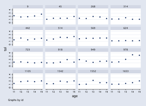
Figure 2.3, page 27.
use https://stats.idre.ucla.edu/stat/stata/examples/alda/data/tolerance_pp, clear

graph twoway (lowess tolerance age)(scatter tolerance age), by(id)

Table 2.2, page 30.
use https://stats.idre.ucla.edu/stat/stata/examples/alda/data/tolerance_pp, clear

statsby _b[_cons] _se[_cons] _b[time] _se[time] (e(rmse)^2) e(r2), by(id) saving(statby): regress tolerance time
(running regress on estimation sample)

      command:  regress tolerance time
      _stat_1:  _b[_cons]
      _stat_2:  _se[_cons]
      _stat_3:  _b[time]
      _stat_4:  _se[time]
      _stat_5:  e(rmse)^2
      _stat_6:  e(r2)
           by:  id

Statsby groups
----+--- 1 ---+--- 2 ---+--- 3 ---+--- 4 ---+--- 5
...............


use statby

list, clean

         id    _stat_1    _stat_2   _stat_3    _stat_4    _stat_5    _stat_6
  1.      9      1.902   .2519484      .119   .1028575   .1057967   .3085185
  2.     45      1.144   .1333567      .174   .0544426     .02964   .7729779
  3.    268      1.536   .2603805      .023   .1062999   .1129967   .0153654
  4.    314      1.306   .1526565      -.03   .0623217     .03884   .0717018
  5.    442      1.576   .2078653      .058   .0848607   .0720133   .1347324
  6.    514       1.43   .1379493      .265   .0563176   .0317167   .8806747
  7.    569      1.816   .0257294      .049    .010504   .0011033   .8788434
  8.    624       1.12        .04       .02   .0163299   .0026667   .3333333
  9.    723      1.268   .0844275     -.054   .0344674     .01188        .45
 10.    918          1   .3044437      .143   .1242886   .1544767   .3061594
 11.    949      1.728   .2411804     -.098   .0984615   .0969467   .2482424
 12.    978      1.028     .31995      .632    .130619   .1706134   .8864112
 13.   1105      1.538   .1511555      .156    .061709     .03808   .6805369
 14.   1542      1.194   .1803275      .237   .0736184   .0541967    .775515
 15.   1552      1.184   .3735532      .153   .1525025     .23257   .2512234
 16.   1653   .9540001   .1392551      .246   .0568507     .03232    .861904
Figure 2.4, page 31.
Note: Use the data that remain in memory after issuing the statsby command in table 2.2.
stem _stat_1, round(.01)  /* _stat_1 is fitted initial status */

   9* | 5
  10* | 03
  11* | 2489
  12* | 7
  13* | 1
  14* | 3
  15* | 448
  16* |
  17* | 3
  18* | 2
  19* | 0

stem _stat_3, round(.01)  /* _stat_3 is fitted rate of change */

 -1* | 0
 -0* | 53
  0* | 2256
  1* | 24567
  2* | 456
  3* |
  4* |
  5* |
  6* | 3

stem _stat_5, round(.01)  /* _stat_5 is residual variance */

  0* | 00133344
  0. | 57
  1* | 011
  1. | 57
  2* | 3

stem _stat_6, round(.01)  /* _stat_6 is r-squared */

  0* | 27
  1* | 3
  2* | 55
  3* | 113
  4* | 5
  5* |
  6* | 8
  7* | 78
  8* | 6889

save statby, replace
Figure 2.5, page 32.
use https://stats.idre.ucla.edu/stat/stata/examples/alda/data/tolerance_pp, clear

graph twoway (lfit tolerance age)(scatter tolerance age), by(id)
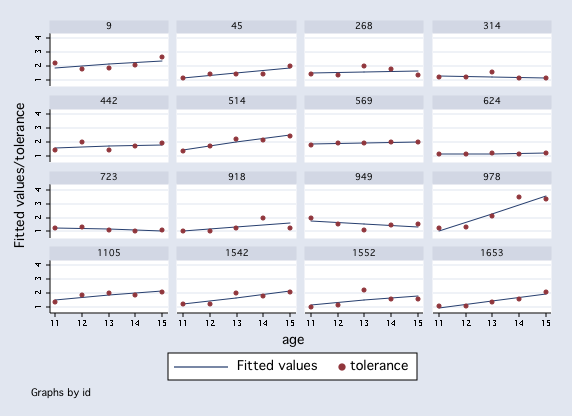
Table 2.3, page 37.
Note: Use the data that remain in memory after issuing the statsby command in table 2.2.
use statby, clear

summarize _stat_1 _stat_3

    Variable |     Obs        Mean   Std. Dev.       Min        Max
-------------+-----------------------------------------------------
     _stat_1 |      16     1.35775   .2977792   .9540001      1.902
     _stat_3 |      16    .1308125   .1722959      -.098       .632

correlate _stat_1 _stat_3
(obs=16)

             |   _stat_1   _stat_3
-------------+---------------------
     _stat_1 |   1.0000
     _stat_3 |  -0.4481   1.0000
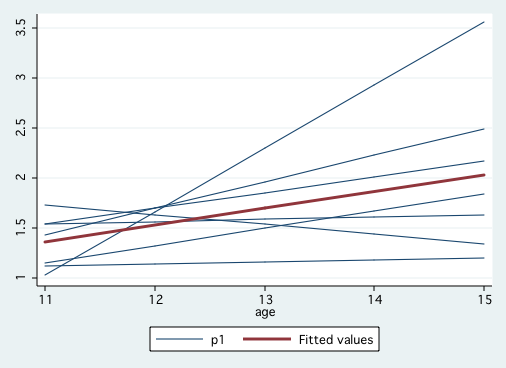
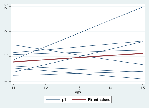
Figure 2.7, page 38.
/* panel 2 */
use https://stats.idre.ucla.edu/stat/stata/examples/alda/data/tolerance_pp, clear
egen grp=group(id)
generate p1=.
forvalues i = 1/16 {
quietly regress tolerance age if grp==`i'
quietly predict p
quietly replace p1=p if grp==`i'
quietly drop p
}
/* panel 1 (labels reversed in book) */
graph twoway (scatter p1 age if ~male, msym(i) connect(L))(lfit tolerance age, lwidth(thick))
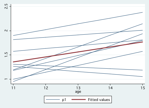 /* panel 2 (labels reversed in book) */
graph twoway (scatter p1 age if male, msym(i) connect(L))(lfit tolerance age, lwidth(thick))
/* panel 2 (labels reversed in book) */
graph twoway (scatter p1 age if male, msym(i) connect(L))(lfit tolerance age, lwidth(thick))
 generate hiexp= exposure>1.145
/* panel 3 */
graph twoway (scatter p1 age if ~hiexp, msym(i) connect(L))(lfit tolerance age if ~hiexp, lwidth(thick))
generate hiexp= exposure>1.145
/* panel 3 */
graph twoway (scatter p1 age if ~hiexp, msym(i) connect(L))(lfit tolerance age if ~hiexp, lwidth(thick))
 /* panel 4 */
graph twoway (scatter p1 age if hiexp, msym(i) connect(L))(lfit tolerance age if hiexp, lwidth(thick))
/* panel 4 */
graph twoway (scatter p1 age if hiexp, msym(i) connect(L))(lfit tolerance age if hiexp, lwidth(thick))
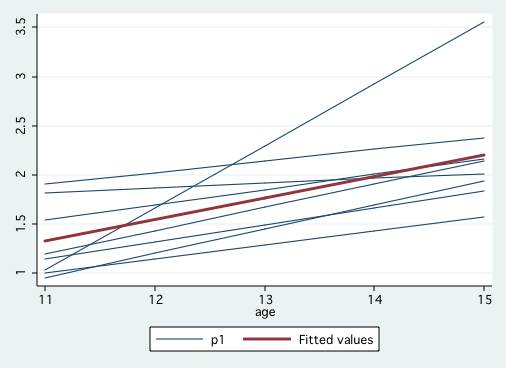
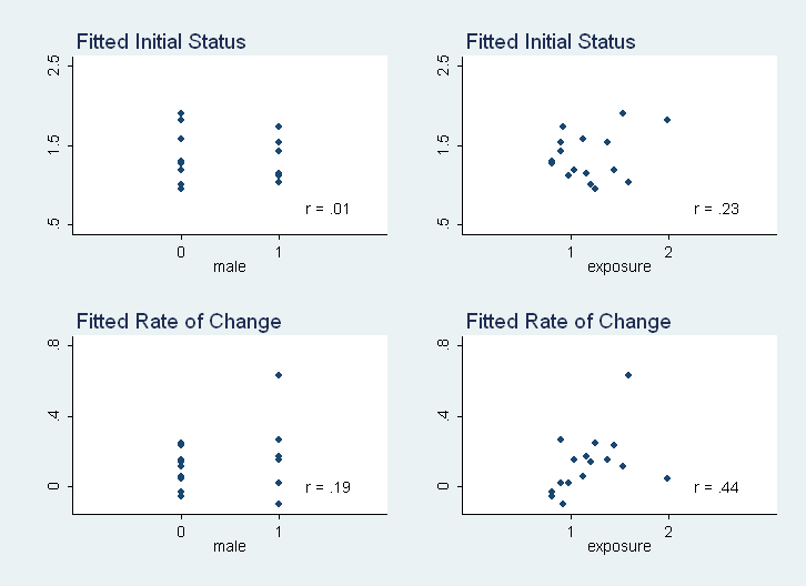
Figure 2.8, page 40.
use https://stats.idre.ucla.edu/stat/stata/examples/alda/data/tolerance, clear
sort id
save tolerance, replace
use https://stats.idre.ucla.edu/stat/stata/examples/alda/data/tolerance_pp, clear
statsby _b[_cons] _se[_cons] _b[time] _se[time] (e(rmse)^2) e(r2), by(id) saving(statby, replace): ///
regress tolerance time
use statby, clear
rename _stat_1 initialfitted
rename _stat_2 initialse
rename _stat_3 changeratefitted
rename _stat_4 changeratese
rename _stat_5 residvariance
rename _stat_6 rsquared
merge id using tolerance
drop _merge

correlate initialfitted male
local rho1=round(r(rho), .01)
graph twoway scatter initialfitted male, xlabel(0 1) ylabel(.5 1.5 2.5, nogrid) ///
title("Fitted Initial Status", position(11)) text(.7 1.5 "r = `rho1'") ytitle(" ") ///
xscale(r(-1 2)) name(g1, replace)

correlate initialfitted exposure
local rho2=round(r(rho), .01)
graph twoway scatter initialfitted exposure, xlabel(1 2) ylabel(.5 1.5 2.5, nogrid) ///
title("Fitted Initial Status", position(11)) text(.7 2.5 "r = `rho2'") ytitle(" ") ///
xscale(r(0 3)) name(g2, replace)

correlate changeratefitted male
local rho3=round(r(rho), .01)
graph twoway scatter changeratefitted male, xlabel(0 1) ylabel(0 .4 .8, nogrid) ///
title("Fitted Rate of Change", position(11)) text(0 1.5 "r = `rho3'") ytitle(" ") ///
xscale(r(-1 2)) name(g3, replace)

correlate changeratefitted exposure
local rho4=round(r(rho), .01)
graph twoway scatter changeratefitted exposure, xlabel(1 2) ylabel(0 .4 .8, nogrid) ///
title("Fitted Rate of Change", position(11)) ytitle(" ") text(0 2.5 "r = `rho4'") ///
xscale(r(0 3)) name(g4, replace)

graph combine g1 g2 g3 g4