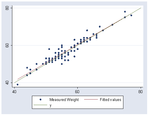
The following shows how to get the graph shown in figure 5.1, page 86.
First, we use the davis file and keep just women.
use https://stats.idre.ucla.edu/stat/stata/examples/ara/davis if female == 1, clear
(From Fox, Applied Regression Analysis.  Use 'notes' command for source of data)
There was an error for subject 12. The measured weight (measwt) and measured height (measht) were switched. Below we fix this by switching them back, just for subject 12.
generate t = measwt if subject==12
(111 missing values generated)

replace measwt = measht if subject==12
(1 real change made)

replace measht = t if subject==12
(1 real change made)

drop t
graph twoway (scatter measwt reptwt) (lfit measwt reptwt) ///
	(function y = x, range(40 80)), xlabel(40 60 80) ylabel(40 60 80)
The following shows how to get the regression equation shown on page 89. This still uses the davis data file we previously used and fixed.
regress measwt reptwt

  Source |       SS       df       MS                  Number of obs =     101
---------+------------------------------               F(  1,    99) = 1024.54
   Model |  4334.88935     1  4334.88935               Prob > F      =  0.0000
Residual |  418.873025    99  4.23104066               R-squared     =  0.9119
---------+------------------------------               Adj R-squared =  0.9110
   Total |  4753.76238   100  47.5376238               Root MSE      =  2.0569

------------------------------------------------------------------------------
  measwt |      Coef.   Std. Err.       t     P>|t|       [95% Conf. Interval]
---------+--------------------------------------------------------------------
  reptwt |   .9772242   .0305301     32.009   0.000       .9166458    1.037803
   _cons |   1.777503   1.744408      1.019   0.311       -1.68378    5.238787
------------------------------------------------------------------------------
To get the Se from page 90, you can just take the square root of MSResidual.
display sqrt(4.231)

2.0569395
The following shows how to get the regression equation shown on Page 100. This uses the duncan data file.
use https://stats.idre.ucla.edu/stat/stata/examples/ara/duncan, clear
(From Fox, Applied Regression Analysis.  Use 'notes' command for source of data)

regress prestige educ income

  Source |       SS       df       MS                  Number of obs =      45
---------+------------------------------               F(  2,    42) =  101.22
   Model |  36180.9458     2  18090.4729               Prob > F      =  0.0000
Residual |  7506.69865    42   178.73092               R-squared     =  0.8282
---------+------------------------------               Adj R-squared =  0.8200
   Total |  43687.6444    44   992.90101               Root MSE      =  13.369

------------------------------------------------------------------------------
prestige |      Coef.   Std. Err.       t     P>|t|       [95% Conf. Interval]
---------+--------------------------------------------------------------------
    educ |   .5458339   .0982526      5.555   0.000       .3475521    .7441158
  income |   .5987328   .1196673      5.003   0.000       .3572343    .8402313
   _cons |  -6.064663   4.271941     -1.420   0.163      -14.68579    2.556463
------------------------------------------------------------------------------
The following shows how to get the regression equation shown on page 102. This uses the prestige data file.
use https://stats.idre.ucla.edu/stat/stata/examples/ara/prestige, clear
(From Fox, Applied Regression Analysis.  Use 'notes' command for source of data )

regress prestige educat income percwomn

  Source |       SS       df       MS                  Number of obs =     102
---------+------------------------------               F(  3,    98) =  129.19
   Model |  23861.8558     3  7953.95195               Prob > F      =  0.0000
Residual |  6033.57026    98  61.5670435               R-squared     =  0.7982
---------+------------------------------               Adj R-squared =  0.7920
   Total |  29895.4261   101  295.994318               Root MSE      =  7.8465

------------------------------------------------------------------------------
prestige |      Coef.   Std. Err.       t     P>|t|       [95% Conf. Interval]
---------+--------------------------------------------------------------------
  educat |   4.186637   .3887013     10.771   0.000       3.415272    4.958002
  income |   .0013136   .0002778      4.729   0.000       .0007623    .0018648
percwomn |  -.0089052   .0304071     -0.293   0.770       -.069247    .0514367
   _cons |  -6.794334   3.239089     -2.098   0.039       -13.2222   -.3664679
------------------------------------------------------------------------------
Page 103 shows how to get the Standard Error from the regression on the duncan data from page 100. You can do this in Stata by taking the square root of the MSResidual from that analysis.
display sqrt(178.73)

13.368994
The bottom of page 103 shows how to get the Standard Error from regression using the prestige data file. You can do this in Stata by taking the square root of the of the MSResidual from that analysis.
display sqrt(61.567)

7.8464642
Page 105 shows how to get the r2 for the regression analyses using the duncan and presige data files. You can simply inspect the tables produced by Stata to see the values of r2 labeled as R-squared.
Page 108 shows how to get standardized regression coefficients for the regression using the prestige data. You can do this in Stata by using the beta option as shown below. The standardized regression coefficients are given in the column labeled Beta.
regress prestige educat income percwomn, beta

  Source |       SS       df       MS                  Number of obs =     102
---------+------------------------------               F(  3,    98) =  129.19
   Model |  23861.8558     3  7953.95195               Prob > F      =  0.0000
Residual |  6033.57026    98  61.5670435               R-squared     =  0.7982
---------+------------------------------               Adj R-squared =  0.7920
   Total |  29895.4261   101  295.994318               Root MSE      =  7.8465

------------------------------------------------------------------------------
prestige |      Coef.   Std. Err.       t     P>|t|                       Beta
---------+--------------------------------------------------------------------
  educat |   4.186637   .3887013     10.771   0.000                   .6639551
  income |   .0013136   .0002778      4.729   0.000                   .3241756
percwomn |  -.0089052   .0304071     -0.293   0.770                   -.016421
   _cons |  -6.794334   3.239089     -2.098   0.039                          .
------------------------------------------------------------------------------

