This page shows how to obtain the results of Fox’s Chapter 2 using Stata. Some of the graphs look somewhat different than those shown in Fox. In some cases, the Stata program is doing something similar to, but not exactly the same as, what is illustrated by Fox.
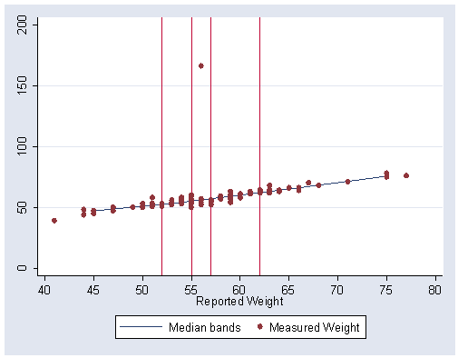
Page 20, figure 2.3. These graphs use medians instead of means, but the commands easily produce very similar plots. bands(5) tells Stata to split the sample into 5 groups for computing the medians.
use https://stats.idre.ucla.edu/stat/stata/examples/ara/davis if female == 1, clear
(From Fox, Applied Regression Analysis.  Use 'notes' command for source of data)

gen c = 1
table c, c(p20 reptwt p40 reptwt p60 reptwt p80 reptwt)

--------------------------------------------------------------
        c | p20(reptwt)  p40(reptwt)  p60(reptwt)  p80(reptwt)
----------+---------------------------------------------------
        1 |          52           55           57           62
--------------------------------------------------------------

graph twoway (mband measwt reptwt, bands(5)) (scatter measwt reptwt), ///
        ylabel(0(50)200) xlabel(40(5)80) xline(52 55 57 62)
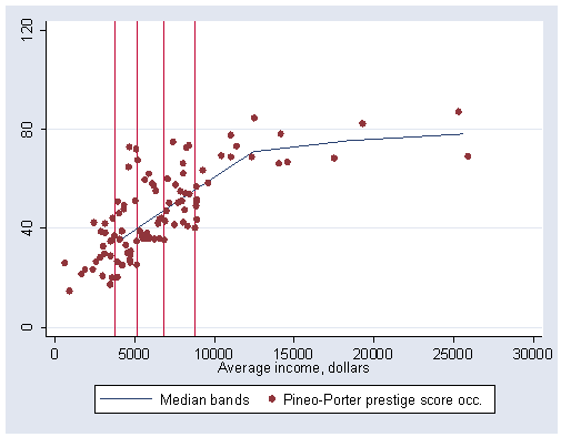
Page 21, figure 2.4 This graphs medians making a figure similar to 2.4. Due to the options chosen by Stata, the graph looks somewhat different.
use https://stats.idre.ucla.edu/stat/stata/examples/ara/prestige, clear
(From Fox, Applied Regression Analysis.  Use 'notes' command for source of data)

gen c = 1
table c, c(p20 income p40 income p60 income p80 income)

--------------------------------------------------------------
        c | p20(income)  p40(income)  p60(income)  p80(income)
----------+---------------------------------------------------
        1 |        3739         5134         6860         8780
--------------------------------------------------------------

graph twoway (mband prestige income, bands(5)) (scatter prestige income), ///
        xlabel(0(5000)30000) ylabel(0(40)120) xline(3739 5134 6860 8780)
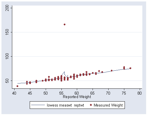
Page 26, figure 2.6. The lowess command is used to get smoothed means. In Fox, the local average is based on 20 observations. The bwidth(.2) command says to use 20% of the data (.20 * 101~=20) for each local average.
use https://stats.idre.ucla.edu/stat/stata/examples/ara/davis, clear

keep if female==1
graph twoway (lowess measwt reptwt, bwidth(.2) noweight mean) ///
	(scatter measwt reptwt), xlabel(40(5)80)
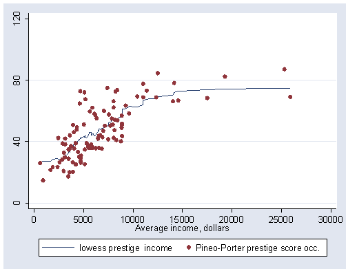
Page 27, figure 2.7. We use the Stata’s lowess command to perform and graph the nonparametric regression.
use https://stats.idre.ucla.edu/stat/stata/examples/ara/prestige, clear

graph twoway (lowess prestige income, bwidth(.2) noweight mean) (scatter prestige income), ///
	xlabel(0(5000)30000) ylabel(0(40)120)
Page 29, figure 2.9 Fox shows figure 2.6 but using the tricube weight function, selected using the locally weighted averages.
use https://stats.idre.ucla.edu/stat/stata/examples/ara/davis, clear

keep if female==1
graph twoway (lowess measwt reptwt, bwidth(.2) mean) (scatter measwt reptwt), xlabel(40(5)80)
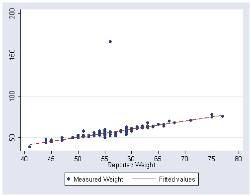
On page 30, figure 2.10 shows the regression using robust regression, using the rreg command. We generate the predicted values using the predict command, and then using the line graph command to show the scatterplot and regression line.
rreg measwt reptwt
predict yhat
graph twoway (scatter measwt reptwt) (line yhat reptwt), xlabel(40(5)80)

