Table 2.1, Table 2.2, and Figure 2.1 on pages 17, 20, and 21. The lean1 scheme is used for the graphs on this page. To download this Stata scheme, use the search command. For these examples, we are entering a dataset.
input subject time censor
  1 6  1
  2 44 1
  3 21 0
  4 14 1
  5 62 1
  end
list, clean

       subject   time   censor
  1.         1      6        1
  2.         2     44        1
  3.         3     21        0
  4.         4     14        1
  5.         5     62        1

stset time, id(subject) failure(censor)
sts list

         failure _d:  censor
   analysis time _t:  time
                 id:  subject

           Beg.          Net            Survivor      Std.
  Time    Total   Fail   Lost           Function     Error     [95% Conf. Int.]
-------------------------------------------------------------------------------
     6        5      1      0             0.8000    0.1789     0.2038    0.9692
    14        4      1      0             0.6000    0.2191     0.1257    0.8818
    21        3      0      1             0.6000    0.2191     0.1257    0.8818
    44        2      1      0             0.3000    0.2387     0.0123    0.7192
    62        1      1      0             0.0000         .          .         .
-------------------------------------------------------------------------------

sts graph, xlabel(0(12)60) ylabel(0(.2)1, nogrid angle(horizontal)) ///
           xtitle(Survival Time) ytitle(Esitmated Survival Probabiltiy) ///
            title(Figure 2.1)

         failure _d:  censor
   analysis time _t:  time
                 id:  subject
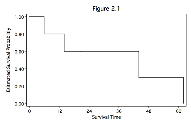
Figure 2.2 on page 22. This graph is generated using the whas100 dataset.
use https://stats.idre.ucla.edu/stat/examples/asa2/whas100, clear
gen fyear=foltime/365.25
stset fyear, id(id) failure(folstatus)
sts graph, xlabel(0(2)8) ylabel(0(.2)1, nogrid angle(horizontal)) ///
            xtitle(Survival Time (Years)) ytitle(Estimated Survival Probability) ///
            title(Figure 2.2)

         failure _d:  folstatus
   analysis time _t:  fyear
                 id:  id
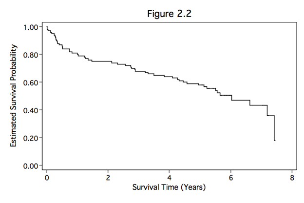
Table 2.3 on page 23 using the whas100 dataset.
stset foltime, fail(folstatus)
sts list, enter

         failure _d:  folstatus
   analysis time _t:  foltime

           Beg.                         Survivor      Std.
  Time    Total   Fail   Lost  Enter    Function     Error     [95% Conf. Int.]
-------------------------------------------------------------------------------
     0        0      0      0    100      1.0000         .          .         .
     6      100      2      0      0      0.9800    0.0140     0.9224    0.9950
    14       98      1      0      0      0.9700    0.0171     0.9099    0.9902
    44       97      1      0      0      0.9600    0.0196     0.8969    0.9848
    62       96      1      0      0      0.9500    0.0218     0.8840    0.9789
    89       95      1      0      0      0.9400    0.0237     0.8713    0.9726

...additional output omitted...

  2641        3      0      1      0      0.3606    0.0857     0.1997    0.5241
  2710        2      1      0      0      0.1803    0.1345     0.0179    0.4820
  2719        1      0      1      0      0.1803    0.1345     0.0179    0.4820
-------------------------------------------------------------------------------
Table 2.4 on page 24 using the whas100 dataset.
stset fyear, id(id) failure(folstatus)
ltable fyear folstatus, saving(ltable1, replace)

                 Beg.                                 Std.
   Interval     Total   Deaths   Lost    Survival    Error     [95% Conf. Int.]
-------------------------------------------------------------------------------
    0     1       100       20      0     0.8000    0.0400     0.7074    0.8660
    1     2        80        5      0     0.7500    0.0433     0.6529    0.8236
    2     3        75        7      0     0.6800    0.0466     0.5790    0.7617
    3     4        68        4      0     0.6400    0.0480     0.5377    0.7254
    4     5        64        6      0     0.5800    0.0494     0.4772    0.6696
    5     6        58        5     39     0.5047    0.0532     0.3965    0.6032
    6     7        14        2      0     0.4326    0.0656     0.3027    0.5556
    7     8        12        2     10     0.3090    0.0875     0.1520    0.4808
-------------------------------------------------------------------------------
Figure 2.3 on page 25. This graph is produced using a dataset created in the previous example (ltable1).
use https://stats.idre.ucla.edu/stat/examples/asa2/ltable1, clear

set obs 9
replace t1=0 in l
replace survival=1 in l
sort t1

twoway line survival t1, con(J) ylabel(0(.2)1) ///
   xlabel(0(2)8) xtitle(Survival Time (Years)) ytitle(Estimated Survival Probability) ///
   title(Figure 2.3)
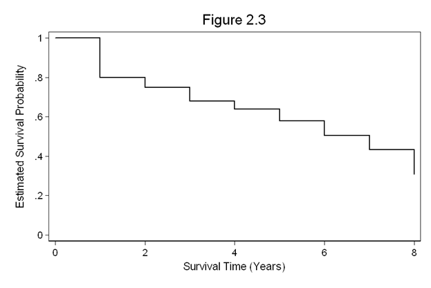
Figure 2.4 on page 26. This graph depicts the polygon representation of the life-table estimate from the dataset in the above example (ltable1).
twoway connect survival t1, msymbol(o) ylabel(0(.2)1) ///
   xlabel(0(2)8) xtitle(Survival Time (Years)) ytitle(Estimated Survival Probability) ///
   title(Figure 2.4)
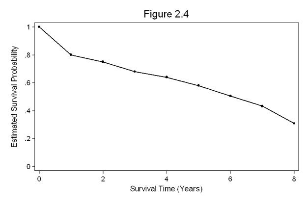
Figure 2.5 on page 31 using the whas100 dataset.
use https://stats.idre.ucla.edu/stat/examples/asa2/whas100, clear
gen fyear = foltime/365.25
stset fyear, id(id) failure(folstatus)
sts gen s=s se=se(s) ub=ub(s) lb=lb(s)
sort fyear

twoway (line s fyear, con(J))(line ub fyear, con(J))(line lb fyear, con(J)), ///
   legend(off) xtitle(Survival Time (Years)) ytitle(Estimated Survival Probability) ///
   title(Figure 2.5)
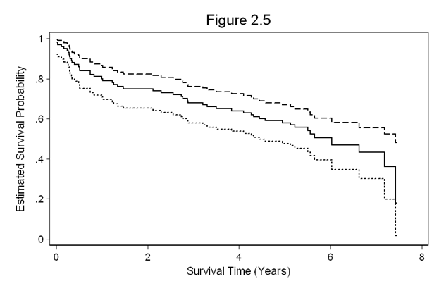
Figure 2.6 on page 32. For this figure, we continue to use the whas100 dataset from the example above.
* log-log transformation
gen ll_s = se/(s*ln(s))
gen ll_l = exp(- exp(ln(-ln(s))  - 1.96*ll_s))
gen ll_u = exp(- exp(ln(-ln(s))  + 1.96*ll_s))

* log transformation, formula 2.3
gen log_s = se/s
gen log_l  = s*exp( - 1.96*log_s)
gen log_u  = s*exp(   1.96*log_s)

* logit transformation. f'=1/(S(t)*(1-S(t))
gen logit_s = se/(s*(1-s))
gen logit_surv = ln(s/(1-s))
gen logit_l   = exp(logit_surv  - 1.96*logit_s)/(1+exp(logit_surv   - 1.96*logit_s))
gen logit_u  = exp(logit_surv  + 1.96*logit_s)/(1+exp(logit_surv + 1.96*logit_s))

* arcsine transformation
gen arcs_s = se/sqrt(1-s^2)
gen arcs_surv = asin(s)

gen arcs_l   = sin(arcs_surv  - 1.96*arcs_s)
gen arcs_u  = sin(arcs_surv + 1.96*arcs_s)

sort fyear
twoway (line s fyear, con(J)) ///
       (line ll_u ll_l fyear, con(J J) lpattern(dash dash) lcolor(black black)) ///
       (line log_u log_l fyear, con(J J) lpattern(dash_dot dash_dot) lcolor(black black)) ///
       (line logit_u logit_l fyear, con(J J) lpattern(longdash longdash) lcolor(black black)) ///
       (line arcs_u arcs_l fyear, con(J J) lpattern(shortdash shortdash) lcolor(black black)), ///
       l2title(Estimated Survival Probability, size(medsmall)) ///
       legend(off) ylabel(,nogrid angle(horizontal)) yscale(titlegap(3)) xscale(titlegap(3)) ///
       xtitle(Survival Time (Years)) title(Figure 2.6)
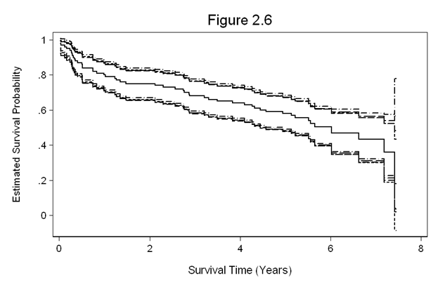
Figure 2.7 on page 34 using the whas100 dataset.
use https://stats.idre.ucla.edu/stat/examples/asa2/whas100, clear
gen fyear = foltime/365.25
stset fyear, failure(folstatus)

sts gen s=s se=se(s) ub=ub(s) lb=lb(s)

* compute the variance of the log of the Kaplan-Meier estimateor
gen sigma2 = se^2/s^2

* what is H_a_alpha in formula (29)?
* compute "a" first. Notice that the largest noncensored vlaue of time is 2710, or 7.42 years
* n = 100 cases
* notice the value for sigma2 when time = 7.42 is .557
* a = 100*557/(1+100*557)
* looking up the table from Appendix 3: we get H = 1.358
gen bl  = ln(-ln(s)) - 1.358*(1+100*sigma2)/(sqrt(100)*ln(s))
gen bu  = ln(-ln(s)) + 1.358*(1+100*sigma2)/(sqrt(100)*ln(s))
gen ebl  = exp(-exp(bu))
gen ebu  = exp(-exp(bl))
gen var2_6 = se^2/(s^2*(ln(s))^2)
gen cl  =ln(-ln(s)) - 1.96*sqrt(var2_6)
gen cu  =ln(-ln(s)) + 1.96*sqrt(var2_6)
gen l = exp(-exp(cu))
gen u = exp(-exp(cl))

sort fyear
twoway (line s fyear, c(J) clcolor(black)) ///
       (line ebl ebu fyear, c(J J) clcolor(black black) clpattern("-..-" "-..-") ) ///
       (line l u fyear,     c(J J) clcolor(black black) clpattern("-" "-")) , ///
        yscale(range(0(0.2)1))  l2title(Estimated Survival Probability, size(medsmall)) ///
        legend( off) ylabel(,nogrid angle(horizontal)) yscale(titlegap(3)) xscale(titlegap(3)) ///
        xtitle(Survival Time (Years)) title(Figure 2.7)
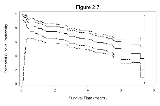
Figure 2.8 on page 35. For this example, we will enter a dataset.
clear
input subject time censor
  1 6  1
  2 44 1
  3 21 0
  4 14 1
  5 62 1
end

stset time, id(subject) failure(censor)

sts graph, scheme(s2mono) xline(14 44, lpattern(dash)) ///
    yline(.25 .5 .75, lpattern(dash)) ///
    ylabel(0(.25)1, angle(0)) ///
    xlabel(0(12)60) xtitle(Survival Time) ytitle(Estimated Survival Probability) ///
    title(Figure 2.8)

         failure _d:  censor
   analysis time _t:  time
                 id:  subject
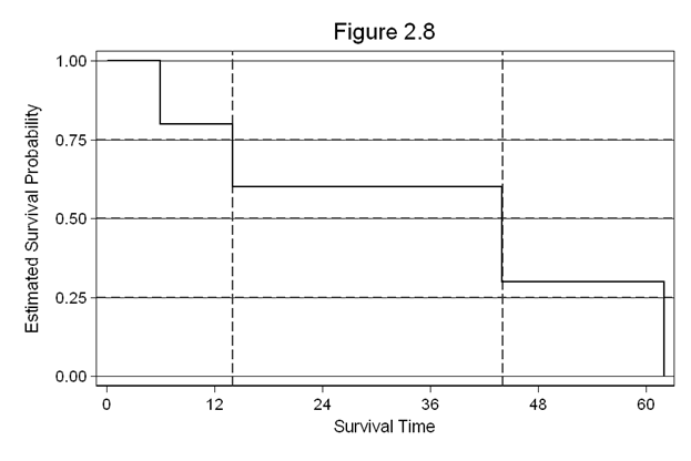
Table 2.5 on page 39. Note that Stata computes the confidence intervals differently from the book.
use https://stats.idre.ucla.edu/stat/examples/asa2/whas100, clear
generate fyear = foltime/365.25
stset fyear, id(id) failure(folstatus)

stsum

         failure _d:  folstatus
   analysis time _t:  fyear
                 id:  id

         |               incidence       no. of    |------ Survival time -----|
         | time at risk     rate        subjects        25%       50%       75%
---------+---------------------------------------------------------------------
   total |   412.156056   .1237395           100   1.472964   6.02601  7.419576

stci

         failure _d:  folstatus
   analysis time _t:  fyear
                 id:  id

             |    no. of
             |  subjects         50%     Std. Err.     [95% Conf. Interval]
-------------+-------------------------------------------------------------
       total |       100     6.02601      .5603603      4.44627    7.41958

stci, p(25)

         failure _d:  folstatus
   analysis time _t:  fyear
                 id:  id

             |    no. of
             |  subjects         25%     Std. Err.     [95% Conf. Interval]
-------------+-------------------------------------------------------------
       total |       100    1.472964      .7682197      .750171    3.29911

stci, p(75)

         failure _d:  folstatus
   analysis time _t:  fyear
                 id:  id

             |    no. of
             |  subjects         75%     Std. Err.     [95% Conf. Interval]
-------------+-------------------------------------------------------------
       total |       100    7.419576      .1409315      7.18412          .
Table 2.6 on page 41. We are using the whas100 dataset from the example above.
sts gen s=s sell=se(lls)
sort fyear
generate z50 = abs(ln(-ln(s))-ln(-ln(.5)))/sell
clist fyear s z50 if z50<1.96 & folstatus==1, noobs
    fyear           s        z50
  4.44627          .6   1.909514
 4.569473         .59   1.726938
 4.944559         .58   1.542441
 5.130733   .56884615   1.331001
 5.221081   .55674304   1.097873
 5.508556   .54036825   .7719651
 5.560575   .52348174   .4438371
 5.653662   .50478596   .0889862
  6.02601   .46872982   .5208178
 6.628337   .43267368   1.042136
 7.184121    .3605614   1.657685
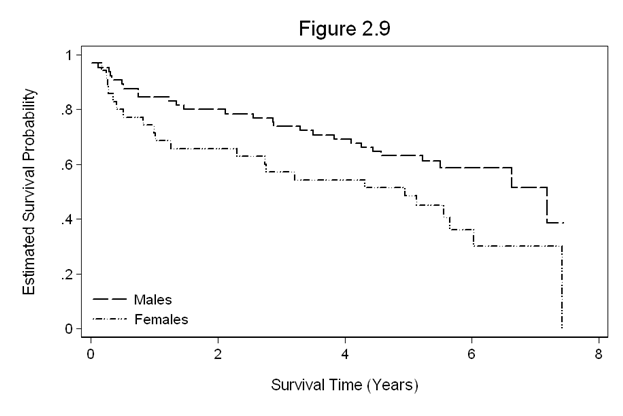
Figure 2.9 on page 46 using the whas100 dataset.
use https://stats.idre.ucla.edu/stat/examples/asa2/whas100.dta, clear
gen fyear=foltime/365.25
stset fyear, fail(folstatus)
sts gen Sm=s  if gender==0
sts gen Sf=s  if gender==1

label variable Sm "Estimated Survival Probability (Males)"
label variable Sf "Estimated Survival Probability (Females)"

sort fyear

scatter Sm Sf fyear, ms( none none) c(J J ) yscale(range(0,1)) clpattern(_ ".-." ) ///
  legend(row(2) col(1) order(1 "Males" 2 "Females") ring(0) position(7)) ///
  ytitle(Estimated Survival Probability)  ylabel(,nogrid angle(horizontal)) ///
  yscale(titlegap(3)) xtitle(Survival Time (Years)) xscale(titlegap(3)) ///
  title(Figure 2.9)
Tables 2.9 and 2.10 on page 50. For this example, we enter in the data found in Table 2.9.
clear
input time d1 n1 d n
  6    0  5  1  9
 14    1  5  1  8
 44    1  4  1  7
 98    1  2  2  4
104    1  1  1  2
114    0  0  1  1
end

gen e1 = n1*d/n
gen v1 =n1*(n-n1)*d*(n-d)/(n^2*(n-1))
replace v1 = 0 if v1==.
gen L = 1
gen W = n
gen T = sqrt(n)

gen P = (n+1-d)/(n+1) in 1
replace P =P[_n-1]*(n+1-d)/(n+1) in 2/l
format e1 v1 L W T P %5.2f
list, noobs clean
    time   d1   n1   d   n     e1     v1      L      W      T      P
       6    0    5   1   9   0.56   0.25   1.00   9.00   3.00   0.90
      14    1    5   1   8   0.63   0.23   1.00   8.00   2.83   0.80
      44    1    4   1   7   0.57   0.24   1.00   7.00   2.65   0.70
      98    1    2   2   4   1.00   0.33   1.00   4.00   2.00   0.42
     104    1    1   1   2   0.50   0.25   1.00   2.00   1.41   0.28
     114    0    0   1   1   0.00   0.00   1.00   1.00   1.00   0.14
Table 2.11 on page 51 using the data above and the formula (2.21) on page 47 showing how the tests are calculated.
tempvar numerator denominator
gen `numerator' = .
gen `denominator' = .

foreach w of varlist L W T P {
   quietly replace `numerator' = `w'*(d1 - e1)
   quietly sum `numerator'
   local t = (r(sum))^2
   quietly replace  `denominator' = `w'^2*v1
   quietly sum `denominator'
   local b = r(sum)
   local Q = `t'/`b'
   local pvalue =chi2tail(1, `Q')
   noisily display "Using weight `w': Q: "   %5.2f  `Q' "  p-value: " %5.2f  `pvalue'
}
Using weight L: Q:  0.43  p-value:  0.51
Using weight W: Q:  0.07  p-value:  0.78
Using weight T: Q:  0.20  p-value:  0.66
Using weight P: Q:  0.11  p-value:  0.75
Table 2.12 on page 51 using the whas100 dataset.
use https://stats.idre.ucla.edu/stat/examples/asa2/whas100.dta,clear
gen fyear=foltime/365.25
stset fyear, fail(folstatus)
sts test gender, logrank

         failure _d:  folstatus
   analysis time _t:  fyear


Log-rank test for equality of survivor functions

       |   Events         Events
gender |  observed       expected
-------+-------------------------
0      |        28          34.62
1      |        23          16.38
-------+-------------------------
Total  |        51          51.00

             chi2(1) =       3.97
             Pr>chi2 =     0.0463

sts test gender, wilcoxon

         failure _d:  folstatus
   analysis time _t:  fyear


Wilcoxon (Breslow) test for equality of survivor functions

       |   Events         Events        Sum of
gender |  observed       expected        ranks
-------+--------------------------------------
0      |        28          34.62         -459
1      |        23          16.38          459
-------+--------------------------------------
Total  |        51          51.00            0

             chi2(1) =       3.46
             Pr>chi2 =     0.0628

sts test gender, tware

         failure _d:  folstatus
   analysis time _t:  fyear


Tarone-Ware test for equality of survivor functions

       |   Events         Events        Sum of
gender |  observed       expected        ranks
-------+--------------------------------------
0      |        28          34.62   -53.311804
1      |        23          16.38    53.311804
-------+--------------------------------------
Total  |        51          51.00            0

             chi2(1) =       3.69
             Pr>chi2 =     0.0549

sts test gender, peto

         failure _d:  folstatus
   analysis time _t:  fyear


Peto-Peto test for equality of survivor functions

       |   Events         Events        Sum of
gender |  observed       expected        ranks
-------+--------------------------------------
0      |        28          34.62   -4.9007719
1      |        23          16.38    4.9007719
-------+--------------------------------------
Total  |        51          51.00            0

             chi2(1) =       3.85
             Pr>chi2 =     0.0497
Table 2.13 on page 52 using the whas100 dataset.
recode age 32/59=1 60/69=2 70/79=3 80/92=4, gen(agecat)
(100 differences between age and agecat)

table agecat, cont(freq sum folstatus)

----------------------------------------
RECODE of |
age       |         Freq.  sum(folsta~s)
----------+-----------------------------
        1 |            25              8
        2 |            23              7
        3 |            22             14
        4 |            30             22
----------------------------------------

stci, by(agecat) median  /* confidence intervals differ from book */

         failure _d:  folstatus
   analysis time _t:  fyear

             |    no. of
agecat       |  subjects         50%     Std. Err.     [95% Conf. Interval]
-------------+-------------------------------------------------------------
           1 |        25           .             .      4.31759          .
           2 |        23    7.184121      .0069868      7.18412          .
           3 |        22    4.944559      .3229116      .750171    6.62834
           4 |        30    2.302532      .9444395       .99384    5.65366
-------------+-------------------------------------------------------------
       total |       100     6.02601      .5603603      4.44627    7.41958
Figure 2.10 on page 55 continuing with the whas100 dataset.
sts gen Sage1=s if age<60
sts gen Sage2=s if age>=60 & age<=69
sts gen Sage3=s if age>=70 & age<=79
sts gen Sage4=s if age>=80

preserve
set obs 101

replace fyear = 0 in 101
replace Sage1 = 1 in 101
replace Sage2 = 1 in 101
replace Sage3 = 1 in 101
replace Sage4 = 1 in 101

sort fyear

scatter Sage1 Sage2 Sage3 Sage4 fyear, ms(none none none none) c(J J J J) ylabel(0(0.2)1) ///
         clpattern(_ ".-."  "-..-" . " -.-") clcolor(black black black black) ///
         legend(row(4) col(1) order(1 "Age < 60" 2 "60 <= Age < 69" 3 "70 <= Age < 79" 4 "Age >=  80") ///
         ring(0) size(medsmall) pos(7) region(lc(white)) ) graphregion(color(white)) ///
         ytitle(Estimated Survival Probability,)  ylabel(,nogrid angle(horizontal)) ///
         yscale(titlegap(3)) xtitle(Survival Time (Years)) xscale(titlegap(3)) title(Figure 2.10)
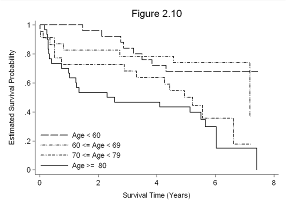
Table 2.15 on page 56 continuing with the whas100 dataset.
restore
sts test agecat, logrank

         failure _d:  folstatus
   analysis time _t:  fyear


Log-rank test for equality of survivor functions

       |   Events         Events
agecat |  observed       expected
-------+-------------------------
1      |         8          15.52
2      |         7          12.92
3      |        14          10.23
4      |        22          12.34
-------+-------------------------
Total  |        51          51.00

             chi2(3) =      15.57
             Pr>chi2 =     0.0014

sts test agecat, wilcoxon

         failure _d:  folstatus
   analysis time _t:  fyear


Wilcoxon (Breslow) test for equality of survivor functions

       |   Events         Events        Sum of
agecat |  observed       expected        ranks
-------+--------------------------------------
1      |         8          15.52         -490
2      |         7          12.92         -385
3      |        14          10.23          201
4      |        22          12.34          674
-------+--------------------------------------
Total  |        51          51.00            0

             chi2(3) =      12.30
             Pr>chi2 =     0.0064

sts test agecat, tware

         failure _d:  folstatus
   analysis time _t:  fyear


Tarone-Ware test for equality of survivor functions

       |   Events         Events        Sum of
agecat |  observed       expected        ranks
-------+--------------------------------------
1      |         8          15.52   -56.455489
2      |         7          12.92   -47.843612
3      |        14          10.23    26.687211
4      |        22          12.34    77.611891
-------+--------------------------------------
Total  |        51          51.00            0

             chi2(3) =      13.52
             Pr>chi2 =     0.0036

sts test agecat, peto

         failure _d:  folstatus
   analysis time _t:  fyear


Peto-Peto test for equality of survivor functions

       |   Events         Events        Sum of
agecat |  observed       expected        ranks
-------+--------------------------------------
1      |         8          15.52   -5.6021925
2      |         7          12.92   -4.0442861
3      |        14          10.23    2.3329794
4      |        22          12.34    7.3134991
-------+--------------------------------------
Total  |        51          51.00            0

             chi2(3) =      14.54
             Pr>chi2 =     0.0023
Table 2.16 on page 57 using the whas100 dataset and the coding scheme defined on page 54.
recode agecat 1=46 2=65 3=75 4 = 86
sts test agecat, logrank trend

         failure _d:  folstatus
   analysis time _t:  fyear


Log-rank test for equality of survivor functions

       |   Events         Events
agecat |  observed       expected
-------+-------------------------
46     |         8          15.52
65     |         7          12.92
75     |        14          10.23
86     |        22          12.34
-------+-------------------------
Total  |        51          51.00

             chi2(3) =      15.57
             Pr>chi2 =     0.0014

Test for trend of survivor functions

             chi2(1) =      12.44
             Pr>chi2 =     0.0004

sts test agecat, wilcoxon trend

         failure _d:  folstatus
   analysis time _t:  fyear


Wilcoxon (Breslow) test for equality of survivor functions

       |   Events         Events        Sum of
agecat |  observed       expected        ranks
-------+--------------------------------------
46     |         8          15.52         -490
65     |         7          12.92         -385
75     |        14          10.23          201
86     |        22          12.34          674
-------+--------------------------------------
Total  |        51          51.00            0

             chi2(3) =      12.30
             Pr>chi2 =     0.0064

Test for trend of survivor functions

             chi2(1) =       9.99
             Pr>chi2 =     0.0016

sts test agecat, tware trend


         failure _d:  folstatus
   analysis time _t:  fyear


Tarone-Ware test for equality of survivor functions

       |   Events         Events        Sum of
agecat |  observed       expected        ranks
-------+--------------------------------------
46     |         8          15.52   -56.455489
65     |         7          12.92   -47.843612
75     |        14          10.23    26.687211
86     |        22          12.34    77.611891
-------+--------------------------------------
Total  |        51          51.00            0

             chi2(3) =      13.52
             Pr>chi2 =     0.0036

Test for trend of survivor functions

             chi2(1) =      10.70
             Pr>chi2 =     0.0011

sts test agecat, peto trend

         failure _d:  folstatus
   analysis time _t:  fyear


Peto-Peto test for equality of survivor functions

       |   Events         Events        Sum of
agecat |  observed       expected        ranks
-------+--------------------------------------
46     |         8          15.52   -5.6021925
65     |         7          12.92   -4.0442861
75     |        14          10.23    2.3329794
86     |        22          12.34    7.3134991
-------+--------------------------------------
Total  |        51          51.00            0

             chi2(3) =      14.54
             Pr>chi2 =     0.0023

Test for trend of survivor functions

             chi2(1) =      12.08
             Pr>chi2 =     0.0005
Figure 2.11 on page 58 using the bpd dataset.
use https://stats.idre.ucla.edu/stat/examples/asa2/bpd, clear

stset ondays, fail(censor)

sts gen s0=s  if surfact==0
sts gen s1=s  if surfact==1

replace s0=1 if s0!=. & ondays==0
replace s1=1 if s1!=. & ondays==0

sts graph, by(surfact) ylabel(0(.2)1) legend( row(2) ring(0) position(1)) ///
   xtitle(Days on Oxygen) ytitle(Estimated Aurvival Probability) ///
   ylabel(, nogrid) title(Figure 2.11)

Table 2.17 on page 58 using the bpd dataset.
sts test suf, logrank

         failure _d:  censor
   analysis time _t:  days


Log-rank test for equality of survivor functions

      |   Events         Events
suf   |  observed       expected
------+-------------------------
0     |        40          48.95
1     |        33          24.05
------+-------------------------
Total |        73          73.00

            chi2(1) =       5.62
            Pr>chi2 =     0.0178

sts test suf, wilcoxon

         failure _d:  censor
   analysis time _t:  days


Wilcoxon (Breslow) test for equality of survivor functions

      |   Events         Events        Sum of
suf   |  observed       expected        ranks
------+--------------------------------------
0     |        40          48.95         -310
1     |        33          24.05          310
------+--------------------------------------
Total |        73          73.00            0

            chi2(1) =       2.49
            Pr>chi2 =     0.1146

sts test suf, tware

         failure _d:  censor
   analysis time _t:  days


Tarone-Ware test for equality of survivor functions

      |   Events         Events        Sum of
suf   |  observed       expected        ranks
------+--------------------------------------
0     |        40          48.95   -50.779103
1     |        33          24.05    50.779103
------+--------------------------------------
Total |        73          73.00            0

            chi2(1) =       3.70
            Pr>chi2 =     0.0545

sts test suf, peto

         failure _d:  censor
   analysis time _t:  days


Peto-Peto test for equality of survivor functions

      |   Events         Events        Sum of
suf   |  observed       expected        ranks
------+--------------------------------------
0     |        40          48.95   -3.9371075
1     |        33          24.05    3.9371075
------+--------------------------------------
Total |        73          73.00            0

            chi2(1) =       2.53
            Pr>chi2 =     0.1114
Figure 2.12 on page 61 using the whas100 dataset.
use https://stats.idre.ucla.edu/stat/examples/asa2/whas100.dta, clear gen fyear = foltime/365.25 stset fyear, fail(folstatus) sts gen skm=s sna=na snalb=lb(na) snaub=ub(na) skmlb=lb(s) skmub=ub(s) replace sna=exp(-sna) replace snaub=exp(-snaub) replace snalb=exp(-snalb) twoway line sna snalb skm skmlb snaub skmub fyear, sort c(J J J J J J) yscale(range(0,1)) /// clpattern(. ".-." - "..-.." ".-." "..-..") /// legend(row(2) col(2) /// order(1 "Nelson-Aalen" 2 "N-A Limits" 3 "Kaplan-Meier" 4 "K-M Limits") /// ring(0) size(medsmall) pos(7) region(lc(white)) ) graphregion(color(white)) /// ytitle(Estimated Survival Probability) ylabel(,nogrid angle(horizontal)) /// yscale(titlegap(3)) xscale(titlegap(3)) xtitle(Survival time (Years)) /// title(Figure 2.12)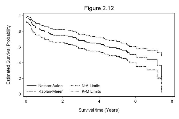
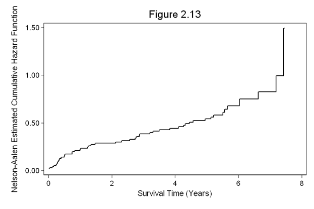
Figure 2.13 on page 62 using the whas100 dataset.sts graph, cumhaz ytitle(Nelson-Aalen Estimated Cumulative Hazard Function) /// xtitle(Survival Time (Years)) ylabel(,nogrid) title(Figure 2.13)
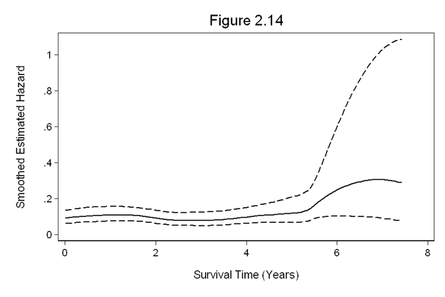
Figure 2.14 on page 64 using the whas100 dataset.
use https://stats.idre.ucla.edu/stat/examples/asa2/whas100.dta, clear gen fyear = foltime/365.25 stset fyear, fail(folstatus) sts graph, hazard cih title(Figure 2.14) xtitle(Survival Time (Years)) /// ytitle("Smoothed Estimated Hazard") ylabel(0(.2)1, nogrid angle(horizontal)) /// yscale(titlegap(3)) xscale(titlegap(3)) noboundary /// legend (off) ciopts(lpattern(dash) lcolor(black) fcolor(none))