Table 4.2 on page 97 using the whas100 dataset.
use https://stats.idre.ucla.edu/stat/examples/asa2/whas100, clear

stset foltime, fail(folstatus)
stcox gender, nohr

         failure _d:  folstatus
   analysis time _t:  foltime

Iteration 0:   log likelihood = -209.11972
Iteration 1:   log likelihood =  -207.2544
Iteration 2:   log likelihood =  -207.2423
Iteration 3:   log likelihood =  -207.2423
Refining estimates:
Iteration 0:   log likelihood =  -207.2423

Cox regression -- Breslow method for ties

No. of subjects =          100                     Number of obs   =       100
No. of failures =           51
Time at risk    =       150540
                                                   LR chi2(1)      =      3.75
Log likelihood  =    -207.2423                     Prob > chi2     =    0.0527

------------------------------------------------------------------------------
          _t |      Coef.   Std. Err.      z    P>|z|     [95% Conf. Interval]
-------------+----------------------------------------------------------------
      gender |   .5554704   .2823858     1.97   0.049     .0020044    1.108936
------------------------------------------------------------------------------
Table 4.3 on page 98 using the actg320 dataset.
use https://stats.idre.ucla.edu/stat/examples/asa2/actg320, clear

stset time, fail(censor)
stcox tx, nohr

         failure _d:  censor
   analysis time _t:  time

Iteration 0:   log likelihood = -658.46549
Iteration 1:   log likelihood = -653.12286
Iteration 2:   log likelihood = -653.11789
Iteration 3:   log likelihood = -653.11789
Refining estimates:
Iteration 0:   log likelihood = -653.11789

Cox regression -- Breslow method for ties

No. of subjects =         1151                     Number of obs   =      1151
No. of failures =           96
Time at risk    =       264941
                                                   LR chi2(1)      =     10.70
Log likelihood  =   -653.11789                     Prob > chi2     =    0.0011

------------------------------------------------------------------------------
          _t |      Coef.   Std. Err.      z    P>|z|     [95% Conf. Interval]
-------------+----------------------------------------------------------------
          tx |  -.6843186   .2149187    -3.18   0.001    -1.105551   -.2630857
------------------------------------------------------------------------------
Table 4.4 on page 99 using the whas100 dataset. We use the groups command, which is user written. To install it, type "ssc install groups" in your command window.
use https://stats.idre.ucla.edu/stat/examples/asa2/whas100, clear

stset foltime, fail(folstatus)
recode age 32/59=1 60/69=2 70/79=3 80/92=4, gen(agecat)

tabulate agecat, gen(age)

  RECODE of |
        age |      Freq.     Percent        Cum.
------------+-----------------------------------
          1 |         25       25.00       25.00
          2 |         23       23.00       48.00
          3 |         22       22.00       70.00
          4 |         30       30.00      100.00
------------+-----------------------------------
      Total |        100      100.00

groups agecat age2 age3 age4 /* search groups */

  +-----------------------------------------------+
  | agecat   age2   age3   age4   Freq.   Percent |
  |-----------------------------------------------|
  |      1      0      0      0      25     25.00 |
  |      2      1      0      0      23     23.00 |
  |      3      0      1      0      22     22.00 |
  |      4      0      0      1      30     30.00 |
  +-----------------------------------------------+
Table 4.5 on page 101 continuing to use the whas100 dataset.
stcox age2 age3 age4, nohr

         failure _d:  folstatus
   analysis time _t:  foltime

Iteration 0:   log likelihood = -209.11972
Iteration 1:   log likelihood = -201.55526
Iteration 2:   log likelihood =  -201.4586
Iteration 3:   log likelihood = -201.45851
Refining estimates:
Iteration 0:   log likelihood = -201.45851

Cox regression -- Breslow method for ties

No. of subjects =          100                     Number of obs   =       100
No. of failures =           51
Time at risk    =       150540
                                                   LR chi2(3)      =     15.32
Log likelihood  =   -201.45851                     Prob > chi2     =    0.0016

------------------------------------------------------------------------------
          _t |      Coef.   Std. Err.      z    P>|z|     [95% Conf. Interval]
-------------+----------------------------------------------------------------
        age2 |   .0468675   .5186444     0.09   0.928    -.9696568    1.063392
        age3 |   .9856007   .4453697     2.21   0.027      .112692    1.858509
        age4 |   1.262993   .4155407     3.04   0.002     .4485481    2.077438
------------------------------------------------------------------------------
Table 4.6 on page 102 continuing to use the whas100 dataset.
stcox age2 age3 age4

         failure _d:  folstatus
   analysis time _t:  foltime

Iteration 0:   log likelihood = -209.11972
Iteration 1:   log likelihood = -201.55526
Iteration 2:   log likelihood =  -201.4586
Iteration 3:   log likelihood = -201.45851
Refining estimates:
Iteration 0:   log likelihood = -201.45851

Cox regression -- Breslow method for ties

No. of subjects =          100                     Number of obs   =       100
No. of failures =           51
Time at risk    =       150540
                                                   LR chi2(3)      =     15.32
Log likelihood  =   -201.45851                     Prob > chi2     =    0.0016

------------------------------------------------------------------------------
          _t | Haz. Ratio   Std. Err.      z    P>|z|     [95% Conf. Interval]
-------------+----------------------------------------------------------------
        age2 |   1.047983   .5435306     0.09   0.928     .3792132    2.896178
        age3 |   2.679421   1.193333     2.21   0.027     1.119287    6.414168
        age4 |   3.535989   1.469347     3.04   0.002     1.566037    7.983985
------------------------------------------------------------------------------
Table 4.7 on page 102 continuing to use the whas100 dataset.
quietly stcox age2 age3 age4, nohr
matrix list e(V), nohalf format(%6.4f)

symmetric e(V)[3,3]
        age2    age3    age4
age2  0.2690  0.1260  0.1251
age3  0.1260  0.1984  0.1260
age4  0.1251  0.1260  0.1727
Table 4.8 on page 105 continuing to use the whas100 dataset. Here, we code the variables using deviations from their means.
foreach var in age2 age3 age4 {
  replace `var'=-1 if agecat==1
  }

stcox age2 age3 age4, nohr

         failure _d:  folstatus
   analysis time _t:  foltime

Iteration 0:   log likelihood = -209.11972
Iteration 1:   log likelihood = -201.55526
Iteration 2:   log likelihood =  -201.4586
Iteration 3:   log likelihood = -201.45851
Refining estimates:
Iteration 0:   log likelihood = -201.45851

Cox regression -- Breslow method for ties

No. of subjects =          100                     Number of obs   =       100
No. of failures =           51
Time at risk    =       150540
                                                   LR chi2(3)      =     15.32
Log likelihood  =   -201.45851                     Prob > chi2     =    0.0016

------------------------------------------------------------------------------
          _t |      Coef.   Std. Err.      z    P>|z|     [95% Conf. Interval]
-------------+----------------------------------------------------------------
        age2 |  -.5269978   .3099716    -1.70   0.089    -1.134531    .0805355
        age3 |   .4117354   .2455778     1.68   0.094    -.0695883    .8930591
        age4 |   .6891276   .2188689     3.15   0.002     .2601526    1.118103
------------------------------------------------------------------------------
Table 4.9 on page 107 continuing to use the whas100 dataset.
stcox age, nohr

         failure _d:  folstatus
   analysis time _t:  foltime

Iteration 0:   log likelihood = -209.11972
Iteration 1:   log likelihood = -200.64424
Iteration 2:   log likelihood = -200.44425
Iteration 3:   log likelihood = -200.44391
Refining estimates:
Iteration 0:   log likelihood = -200.44391

Cox regression -- Breslow method for ties

No. of subjects =          100                     Number of obs   =       100
No. of failures =           51
Time at risk    =       150540
                                                   LR chi2(1)      =     17.35
Log likelihood  =   -200.44391                     Prob > chi2     =    0.0000

------------------------------------------------------------------------------
          _t |      Coef.   Std. Err.      z    P>|z|     [95% Conf. Interval]
-------------+----------------------------------------------------------------
         age |   .0456618   .0119506     3.82   0.000     .0222391    .0690844
------------------------------------------------------------------------------
Table 4.10 on page 107 using the actg320 dataset.
use https://stats.idre.ucla.edu/stat/examples/asa2/actg320, clear

stset time, fail(censor)
stcox cd4, nohr

         failure _d:  censor
   analysis time _t:  time

Iteration 0:   log likelihood = -658.46549
Iteration 1:   log likelihood = -629.94428
Iteration 2:   log likelihood = -626.73801
Iteration 3:   log likelihood = -626.63616
Iteration 4:   log likelihood =   -626.636
Refining estimates:
Iteration 0:   log likelihood =   -626.636

Cox regression -- Breslow method for ties

No. of subjects =         1151                     Number of obs   =      1151
No. of failures =           96
Time at risk    =       264941
                                                   LR chi2(1)      =     63.66
Log likelihood  =     -626.636                     Prob > chi2     =    0.0000

------------------------------------------------------------------------------
          _t |      Coef.   Std. Err.      z    P>|z|     [95% Conf. Interval]
-------------+----------------------------------------------------------------
         cd4 |  -.0161921   .0025026    -6.47   0.000    -.0210971   -.0112872
------------------------------------------------------------------------------
Table 4.11 on page 113 using the gbcs dataset.
use https://stats.idre.ucla.edu/stat/examples/asa2/gbcs, clear

stset rectime, fail(censrec)
generate hormonexsize = hormone*size

stcox hormone, nohr

         failure _d:  censrec
   analysis time _t:  rectime

Iteration 0:   log likelihood = -1788.1731
Iteration 1:   log likelihood =  -1783.774
Iteration 2:   log likelihood =  -1783.765
Iteration 3:   log likelihood =  -1783.765
Refining estimates:
Iteration 0:   log likelihood =  -1783.765

Cox regression -- Breslow method for ties

No. of subjects =          686                     Number of obs   =       686
No. of failures =          299
Time at risk    =       771400
                                                   LR chi2(1)      =      8.82
Log likelihood  =    -1783.765                     Prob > chi2     =    0.0030

------------------------------------------------------------------------------
          _t |      Coef.   Std. Err.      z    P>|z|     [95% Conf. Interval]
-------------+----------------------------------------------------------------
     hormone |  -.3638988   .1250441    -2.91   0.004    -.6089808   -.1188167
------------------------------------------------------------------------------

stcox hormone size, nohr

         failure _d:  censrec
   analysis time _t:  rectime

Iteration 0:   log likelihood = -1788.1731
Iteration 1:   log likelihood = -1776.0514
Iteration 2:   log likelihood = -1775.6959
Iteration 3:   log likelihood = -1775.6954
Refining estimates:
Iteration 0:   log likelihood = -1775.6954

Cox regression -- Breslow method for ties

No. of subjects =          686                     Number of obs   =       686
No. of failures =          299
Time at risk    =       771400
                                                   LR chi2(2)      =     24.96
Log likelihood  =   -1775.6954                     Prob > chi2     =    0.0000

------------------------------------------------------------------------------
          _t |      Coef.   Std. Err.      z    P>|z|     [95% Conf. Interval]
-------------+----------------------------------------------------------------
     hormone |  -.3734745    .125176    -2.98   0.003    -.6188149   -.1281341
        size |   .0152507   .0035639     4.28   0.000     .0082657    .0222358
------------------------------------------------------------------------------

stcox hormone size hormonexsize, nohr

         failure _d:  censrec
   analysis time _t:  rectime

Iteration 0:   log likelihood = -1788.1731
Iteration 1:   log likelihood = -1776.1541
Iteration 2:   log likelihood = -1775.6918
Iteration 3:   log likelihood = -1775.6912
Iteration 4:   log likelihood = -1775.6912
Refining estimates:
Iteration 0:   log likelihood = -1775.6912

Cox regression -- Breslow method for ties

No. of subjects =          686                     Number of obs   =       686
No. of failures =          299
Time at risk    =       771400
                                                   LR chi2(3)      =     24.96
Log likelihood  =   -1775.6912                     Prob > chi2     =    0.0000

------------------------------------------------------------------------------
          _t |      Coef.   Std. Err.      z    P>|z|     [95% Conf. Interval]
-------------+----------------------------------------------------------------
     hormone |  -.3941755   .2601893    -1.51   0.130    -.9041372    .1157862
        size |   .0149727   .0047047     3.18   0.001     .0057515    .0241938
hormonexsize |   .0006522   .0071812     0.09   0.928    -.0134227    .0147272
------------------------------------------------------------------------------
Table 4.12 on page 114 using the uis dataset.
use https://stats.idre.ucla.edu/stat/examples/asa2/uis, clear

stset time, fail(censor)
drop if age==.
drop if ivhx==.

generate drug = ivhx==2 | ivhx==3
generate drugxage = drug*age

stcox drug, nohr

         failure _d:  censor
   analysis time _t:  time

Iteration 0:   log likelihood = -2831.8568
Iteration 1:   log likelihood = -2825.9716
Iteration 2:   log likelihood = -2825.9664
Refining estimates:
Iteration 0:   log likelihood = -2825.9664

Cox regression -- Breslow method for ties

No. of subjects =          605                     Number of obs   =       605
No. of failures =          489
Time at risk    =       144822
                                                   LR chi2(1)      =     11.78
Log likelihood  =   -2825.9664                     Prob > chi2     =    0.0006

------------------------------------------------------------------------------
          _t |      Coef.   Std. Err.      z    P>|z|     [95% Conf. Interval]
-------------+----------------------------------------------------------------
        drug |   .3210045   .0948107     3.39   0.001     .1351789    .5068301
------------------------------------------------------------------------------

stcox drug age, nohr

         failure _d:  censor
   analysis time _t:  time

Iteration 0:   log likelihood = -2831.8568
Iteration 1:   log likelihood = -2820.2006
Iteration 2:   log likelihood = -2820.1989
Refining estimates:
Iteration 0:   log likelihood = -2820.1989

Cox regression -- Breslow method for ties

No. of subjects =          605                     Number of obs   =       605
No. of failures =          489
Time at risk    =       144822
                                                   LR chi2(2)      =     23.32
Log likelihood  =   -2820.1989                     Prob > chi2     =    0.0000

------------------------------------------------------------------------------
          _t |      Coef.   Std. Err.      z    P>|z|     [95% Conf. Interval]
-------------+----------------------------------------------------------------
        drug |   .4394466   .1007151     4.36   0.000     .2420487    .6368445
         age |  -.0263792   .0078392    -3.37   0.001    -.0417438   -.0110147
------------------------------------------------------------------------------

stcox drug age drugxage, nohr

         failure _d:  censor
   analysis time _t:  time

Iteration 0:   log likelihood = -2831.8568
Iteration 1:   log likelihood = -2820.0329
Iteration 2:   log likelihood = -2819.8471
Iteration 3:   log likelihood = -2819.8471
Iteration 4:   log likelihood = -2819.8471
Refining estimates:
Iteration 0:   log likelihood = -2819.8471

Cox regression -- Breslow method for ties

No. of subjects =          605                     Number of obs   =       605
No. of failures =          489
Time at risk    =       144822
                                                   LR chi2(3)      =     24.02
Log likelihood  =   -2819.8471                     Prob > chi2     =    0.0000

------------------------------------------------------------------------------
          _t |      Coef.   Std. Err.      z    P>|z|     [95% Conf. Interval]
-------------+----------------------------------------------------------------
        drug |  -.0124116   .5484471    -0.02   0.982    -1.087348    1.062525
         age |  -.0372282   .0152309    -2.44   0.015    -.0670801   -.0073762
    drugxage |   .0148441   .0177607     0.84   0.403    -.0199662    .0496543
------------------------------------------------------------------------------
Table 4.13 on page 116 using the whas500 dataset.
use https://stats.idre.ucla.edu/stat/examples/asa2/whas500, clear

stset lenfol, fail(fstat)
generate genderxage = gender*age

stcox gender, nohr

         failure _d:  fstat
   analysis time _t:  lenfol

Iteration 0:   log likelihood =  -1227.579
Iteration 1:   log likelihood = -1223.7894
Iteration 2:   log likelihood = -1223.7851
Refining estimates:
Iteration 0:   log likelihood = -1223.7851

Cox regression -- Breslow method for ties

No. of subjects =          500                     Number of obs   =       500
No. of failures =          215
Time at risk    =       441218
                                                   LR chi2(1)      =      7.59
Log likelihood  =   -1223.7851                     Prob > chi2     =    0.0059

------------------------------------------------------------------------------
          _t |      Coef.   Std. Err.      z    P>|z|     [95% Conf. Interval]
-------------+----------------------------------------------------------------
      gender |   .3812532    .137584     2.77   0.006     .1115935    .6509128
------------------------------------------------------------------------------

stcox gender age, nohr

         failure _d:  fstat
   analysis time _t:  lenfol

Iteration 0:   log likelihood =  -1227.579
Iteration 1:   log likelihood = -1158.4911
Iteration 2:   log likelihood =  -1156.574
Iteration 3:   log likelihood = -1156.5702
Refining estimates:
Iteration 0:   log likelihood = -1156.5702

Cox regression -- Breslow method for ties

No. of subjects =          500                     Number of obs   =       500
No. of failures =          215
Time at risk    =       441218
                                                   LR chi2(2)      =    142.02
Log likelihood  =   -1156.5702                     Prob > chi2     =    0.0000

------------------------------------------------------------------------------
          _t |      Coef.   Std. Err.      z    P>|z|     [95% Conf. Interval]
-------------+----------------------------------------------------------------
      gender |  -.0655551   .1405742    -0.47   0.641    -.3410755    .2099653
         age |   .0668283   .0061941    10.79   0.000      .054688    .0789686
------------------------------------------------------------------------------

stcox gender age genderxage, nohr basehc(h)

         failure _d:  fstat
   analysis time _t:  lenfol

Iteration 0:   log likelihood =  -1227.579
Iteration 1:   log likelihood = -1157.5688
Iteration 2:   log likelihood = -1153.7302
Iteration 3:   log likelihood = -1153.6663
Iteration 4:   log likelihood = -1153.6663
Refining estimates:
Iteration 0:   log likelihood = -1153.6663

Cox regression -- Breslow method for ties

No. of subjects =          500                     Number of obs   =       500
No. of failures =          215
Time at risk    =       441218
                                                   LR chi2(3)      =    147.83
Log likelihood  =   -1153.6663                     Prob > chi2     =    0.0000

------------------------------------------------------------------------------
          _t |      Coef.   Std. Err.      z    P>|z|     [95% Conf. Interval]
-------------+----------------------------------------------------------------
      gender |   2.328526   .9923413     2.35   0.019     .3835728    4.273479
         age |   .0784022   .0080213     9.77   0.000     .0626807    .0941236
  genderxage |  -.0304264   .0125362    -2.43   0.015    -.0549968   -.0058559
------------------------------------------------------------------------------
Figure 4.2 on page 117 continuing to use the whas500 dataset and the model above. The graphs shown on this page use the lean1 scheme.
predict hr1, hr

generate lnhr = ln(hr1)

twoway (line lnhr age if gender==0)(line lnhr age if gender==1), ///
   xtitle(Age in Years) ytitle(Estimated Log Hazard) title(Figure 4.2) ///
   ylabel(2(1)8) legend(order(1 "Males" 2 "Females") ring(0) position(11))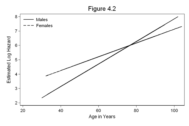
Figure 4.3 on page 118 continuing to use the whas500 dataset. The calculations performed are from equations 4.19-4.22.
matrix V=e(V)
gen ln_hr=_b[gender]+_b[genderxage]*age
replace hr=exp(ln_hr)
gen SE_ln_hr=sqrt(V[1,1]+2*age*V[3,1]+age^2*V[3,3])
gen ln_hr_l=ln_hr-1.96*SE_ln_hr
gen ln_hr_u=ln_hr+1.96*SE_ln_hr

twoway line ln_hr ln_hr_l ln_hr_u age, sort clpattern(l shortdash shortdash ) ///
   clcolor(black black black ) ///
   legend(row(2) col(1) pos(7) order(1 "Log Hazard Ratio"  2 "Confidence Limits")  ///
   ring(0) size(medsmall) region(lc(white)) ) graphregion(color(white))  ///
   yline(0, lcolor(black)) yaxis(1 2) ytitle(Estimated Log Hazard Ratio)  ///
   ylabel(-1(0.5)2.5, nogrid angle(horizontal)) xscale(titlegap(3)) ///
   xtitle(Age in Years) ylabel(, axis(2) angle(horizontal)) ///
   ylabel(-.69 "0.5" 0 "1" .69 "2.0" 1.39 "4.0" 2.30 "10.0", axis(2)) ///
   ytitle(Estimated Hazard Ratio, axis(2)) ///
   yscale(titlegap(3) axis(2)) yscale(titlegap(3) axis(1)) ///
   title(Figure 4.3)
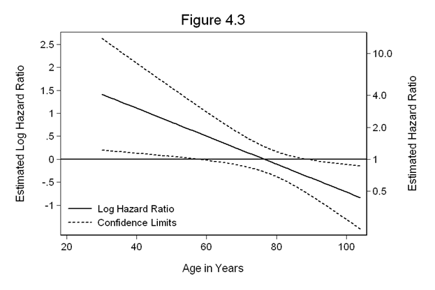
Table 4.14 on page 118 continuing to use the whas500 dataset.
lincom _b[gender]+_b[genderxage]*40, hr

 ( 1)  gender + 40 genderxage = 0

------------------------------------------------------------------------------
          _t | Haz. Ratio   Std. Err.      z    P>|z|     [95% Conf. Interval]
-------------+----------------------------------------------------------------
         (1) |   3.038824    1.52132     2.22   0.026     1.139122    8.106639
------------------------------------------------------------------------------

lincom _b[gender]+_b[genderxage]*50, hr

 ( 1)  gender + 50 genderxage = 0

------------------------------------------------------------------------------
          _t | Haz. Ratio   Std. Err.      z    P>|z|     [95% Conf. Interval]
-------------+----------------------------------------------------------------
         (1) |   2.241638   .8555832     2.11   0.034     1.060916    4.736419
------------------------------------------------------------------------------

lincom _b[gender]+_b[genderxage]*60, hr

 ( 1)  gender + 60 genderxage = 0

------------------------------------------------------------------------------
          _t | Haz. Ratio   Std. Err.      z    P>|z|     [95% Conf. Interval]
-------------+----------------------------------------------------------------
         (1) |   1.653581   .4441904     1.87   0.061     .9767261    2.799484
------------------------------------------------------------------------------

lincom _b[gender]+_b[genderxage]*65, hr

 ( 1)  gender + 65 genderxage = 0

------------------------------------------------------------------------------
          _t | Haz. Ratio   Std. Err.      z    P>|z|     [95% Conf. Interval]
-------------+----------------------------------------------------------------
         (1) |   1.420219   .3085033     1.61   0.106     .9278022    2.173979
------------------------------------------------------------------------------

lincom _b[gender]+_b[genderxage]*85, hr

 ( 1)  gender + 85 genderxage = 0

------------------------------------------------------------------------------
          _t | Haz. Ratio   Std. Err.      z    P>|z|     [95% Conf. Interval]
-------------+----------------------------------------------------------------
         (1) |   .7728143    .124304    -1.60   0.109     .5638492    1.059223
------------------------------------------------------------------------------

lincom _b[gender]+_b[genderxage]*90, hr

 ( 1)  gender + 90 genderxage = 0

------------------------------------------------------------------------------
          _t | Haz. Ratio   Std. Err.      z    P>|z|     [95% Conf. Interval]
-------------+----------------------------------------------------------------
         (1) |   .6637509   .1330606    -2.04   0.041     .4480915    .9832037
------------------------------------------------------------------------------
Table 4.15 on page 199 using the gbcs dataset.
use https://stats.idre.ucla.edu/stat/examples/asa2/gbcs, clear

stset rectime, fail(censrec)
generate hormonexnodes = hormone*nodes

stcox hormone, nohr

         failure _d:  censrec
   analysis time _t:  rectime

Iteration 0:   log likelihood = -1788.1731
Iteration 1:   log likelihood =  -1783.774
Iteration 2:   log likelihood =  -1783.765
Iteration 3:   log likelihood =  -1783.765
Refining estimates:
Iteration 0:   log likelihood =  -1783.765

Cox regression -- Breslow method for ties

No. of subjects =          686                     Number of obs   =       686
No. of failures =          299
Time at risk    =       771400
                                                   LR chi2(1)      =      8.82
Log likelihood  =    -1783.765                     Prob > chi2     =    0.0030

------------------------------------------------------------------------------
          _t |      Coef.   Std. Err.      z    P>|z|     [95% Conf. Interval]
-------------+----------------------------------------------------------------
     hormone |  -.3638988   .1250441    -2.91   0.004    -.6089808   -.1188167
------------------------------------------------------------------------------

stcox hormone nodes, nohr

         failure _d:  censrec
   analysis time _t:  rectime

Iteration 0:   log likelihood = -1788.1731
Iteration 1:   log likelihood = -1759.9643
Iteration 2:   log likelihood = -1758.9415
Iteration 3:   log likelihood = -1758.9407
Refining estimates:
Iteration 0:   log likelihood = -1758.9407

Cox regression -- Breslow method for ties

No. of subjects =          686                     Number of obs   =       686
No. of failures =          299
Time at risk    =       771400
                                                   LR chi2(2)      =     58.46
Log likelihood  =   -1758.9407                     Prob > chi2     =    0.0000

------------------------------------------------------------------------------
          _t |      Coef.   Std. Err.      z    P>|z|     [95% Conf. Interval]
-------------+----------------------------------------------------------------
     hormone |  -.3569371   .1252197    -2.85   0.004    -.6023632    -.111511
       nodes |   .0576747   .0066566     8.66   0.000     .0446281    .0707213
------------------------------------------------------------------------------

stcox hormone nodes hormonexnodes, nohr

         failure _d:  censrec
   analysis time _t:  rectime

Iteration 0:   log likelihood = -1788.1731
Iteration 1:   log likelihood = -1758.5113
Iteration 2:   log likelihood = -1755.9822
Iteration 3:   log likelihood =  -1755.971
Iteration 4:   log likelihood =  -1755.971
Refining estimates:
Iteration 0:   log likelihood =  -1755.971

Cox regression -- Breslow method for ties

No. of subjects =          686                     Number of obs   =       686
No. of failures =          299
Time at risk    =       771400
                                                   LR chi2(3)      =     64.40
Log likelihood  =    -1755.971                     Prob > chi2     =    0.0000

------------------------------------------------------------------------------
          _t |      Coef.   Std. Err.      z    P>|z|     [95% Conf. Interval]
-------------+----------------------------------------------------------------
     hormone |  -.6059966   .1635048    -3.71   0.000    -.9264602    -.285533
       nodes |   .0492431   .0081727     6.03   0.000     .0332249    .0652614
hormonexno~s |   .0381956   .0149761     2.55   0.011     .0088429    .0675483
------------------------------------------------------------------------------
Figure 4.4 on page 120 continuing to use the gbcs dataset. We will use the predicted values and the variance-covariance matrix from the model above to generate the figure.
predict hr1, hr
generate lnhr = ln(hr1)

matrix V=e(V)
gen ln_hr=_b[hormone]+_b[hormonexnodes]*nodes
replace hr=exp(ln_hr)
gen SE_ln_hr=sqrt(V[1,1]+2*nodes*V[3,1]+nodes^2*V[3,3])
gen ln_hr_l=ln_hr-1.96*SE_ln_hr
gen ln_hr_u=ln_hr+1.96*SE_ln_hr

twoway line ln_hr ln_hr_l ln_hr_u nodes, sort clpattern(l shortdash shortdash ) ///
   clcolor(black black black ) ///
   legend(row(2) col(1) pos(11) order(1 "Log Hazard Ratio"  2 "Confidence Limits")  ///
   ring(0) size(medsmall) region(lc(white)) ) graphregion(color(white))  ///
   yline(0, lcolor(black)) yaxis(1 2) ytitle(Estimated Log Hazard Ratio)  ///
   ylabel(-1(0.5)2.5, nogrid angle(horizontal)) xscale(titlegap(3)) ///
   xtitle(Number of Nodes) ylabel(, axis(2) angle(horizontal)) ///
   ylabel(-.69 "0.5" 0 "1" 1.39 "4.0" 2.71 "15.0", axis(2)) ///
   ytitle(Estimated Hazard Ratio, axis(2)) ///
   yscale(titlegap(3) axis(2)) yscale(titlegap(3) axis(1)) ///
   title(Figure 4.4)
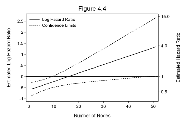
Table 4.16 on page 120 continuing to use the gbcs dataset.
lincom _b[hormone]+_b[hormonexnodes]*1, hr

 ( 1)  hormone + hormonexnodes = 0

------------------------------------------------------------------------------
          _t | Haz. Ratio   Std. Err.      z    P>|z|     [95% Conf. Interval]
-------------+----------------------------------------------------------------
         (1) |   .5667704   .0874547    -3.68   0.000      .418855     .766921
------------------------------------------------------------------------------

lincom _b[hormone]+_b[hormonexnodes]*3, hr

 ( 1)  hormone + 3 hormonexnodes = 0

------------------------------------------------------------------------------
          _t | Haz. Ratio   Std. Err.      z    P>|z|     [95% Conf. Interval]
-------------+----------------------------------------------------------------
         (1) |   .6117633    .085004    -3.54   0.000     .4659183    .8032619
------------------------------------------------------------------------------

lincom _b[hormone]+_b[hormonexnodes]*5, hr

 ( 1)  hormone + 5 hormonexnodes = 0

------------------------------------------------------------------------------
          _t | Haz. Ratio   Std. Err.      z    P>|z|     [95% Conf. Interval]
-------------+----------------------------------------------------------------
         (1) |    .660328   .0850732    -3.22   0.001      .512974      .85001
------------------------------------------------------------------------------

lincom _b[hormone]+_b[hormonexnodes]*7, hr

 ( 1)  hormone + 7 hormonexnodes = 0

------------------------------------------------------------------------------
          _t | Haz. Ratio   Std. Err.      z    P>|z|     [95% Conf. Interval]
-------------+----------------------------------------------------------------
         (1) |    .712748   .0892621    -2.70   0.007      .557615    .9110402
------------------------------------------------------------------------------

lincom _b[hormone]+_b[hormonexnodes]*9, hr
 ( 1)  hormone + 9 hormonexnodes = 0

------------------------------------------------------------------------------
          _t | Haz. Ratio   Std. Err.      z    P>|z|     [95% Conf. Interval]
-------------+----------------------------------------------------------------
         (1) |   .7693293   .0990145    -2.04   0.042     .5978065    .9900654
------------------------------------------------------------------------------
Table 4.17 on page 121 continuing to use the gbcs dataset.
stcox hormone, nohr


         failure _d:  censrec
   analysis time _t:  rectime

Iteration 0:   log likelihood = -1788.1731
Iteration 1:   log likelihood =  -1783.774
Iteration 2:   log likelihood =  -1783.765
Iteration 3:   log likelihood =  -1783.765
Refining estimates:
Iteration 0:   log likelihood =  -1783.765

Cox regression -- Breslow method for ties

No. of subjects =          686                     Number of obs   =       686
No. of failures =          299
Time at risk    =       771400
                                                   LR chi2(1)      =      8.82
Log likelihood  =    -1783.765                     Prob > chi2     =    0.0030

------------------------------------------------------------------------------
          _t |      Coef.   Std. Err.      z    P>|z|     [95% Conf. Interval]
-------------+----------------------------------------------------------------
     hormone |  -.3638988   .1250441    -2.91   0.004    -.6089808   -.1188167
------------------------------------------------------------------------------
Figure 4.5 on page 123 continuing to use the gbcs dataset.
gen months = rectime / 30.4
stset months, fail(censrec)
quietly stcox hormone, nohr basesurv(s45)

gen s45_h = s45^(exp(-.364))
sort months
twoway line s45 s45_h months, ///
   legend(row(2) col(1) pos(7) order(1 "No Hormone Therapy"  2 "Hormone Therapy") ///
   ring(0) size(medsmall))  ///
   ylabel(0(0.2)1) ///
   xtitle(Recurrence Time (Months)) ///
   ytitle(Covariate Adjusted Survival Function) ///
   title(Figure 4.5)

Table 4.18 on page 124 using the gbcs dataset.
stcox hormone size, nohr

         failure _d:  censrec
   analysis time _t:  rectime

Iteration 0:   log likelihood = -1788.1731
Iteration 1:   log likelihood =  -1783.774
Iteration 2:   log likelihood =  -1783.765
Iteration 3:   log likelihood =  -1783.765
Refining estimates:
Iteration 0:   log likelihood =  -1783.765

Cox regression -- Breslow method for ties

No. of subjects =          686                     Number of obs   =       686
No. of failures =          299
Time at risk    =       771400
                                                   LR chi2(1)      =      8.82
Log likelihood  =    -1783.765                     Prob > chi2     =    0.0030

------------------------------------------------------------------------------
          _t |      Coef.   Std. Err.      z    P>|z|     [95% Conf. Interval]
-------------+----------------------------------------------------------------
     hormone |  -.3638988   .1250441    -2.91   0.004    -.6089808   -.1188167
------------------------------------------------------------------------------
Figure 4.6 on page 125 continuing to use the gbcs dataset.
gen size_c = size-25
quietly stcox hormone size_c, nohr basesurv(s46)

gen s46_h = s46^(exp(-.373))
sort months
twoway line s46 s46_h months, ///
   legend(row(2) col(1) pos(7) order(1 "No Hormone Therapy"  2 "Hormone Therapy") ///
   ring(0) size(medsmall))  ///
   ylabel(0(0.2)1) ///
   xtitle(Recurrence Time (Months)) ///
   ytitle(Covariate Adjusted Survival Function) ///
   title(Figure 4.6)
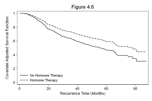
Table 4.19 on page 126 continuing to use the gbcs dataset.
tabulate grade, gen(grade)

      grade |      Freq.     Percent        Cum.
------------+-----------------------------------
          1 |         81       11.81       11.81
          2 |        444       64.72       76.53
          3 |        161       23.47      100.00
------------+-----------------------------------
      Total |        686      100.00

generate ln_prg=ln(prog_recp+1)

stcox hormone grade2 grade3 size ln_prg, nohr


         failure _d:  censrec
   analysis time _t:  rectime

Iteration 0:   log likelihood = -1788.1731
Iteration 1:   log likelihood = -1750.0796
Iteration 2:   log likelihood =  -1748.986
Iteration 3:   log likelihood = -1748.9843
Iteration 4:   log likelihood = -1748.9843
Refining estimates:
Iteration 0:   log likelihood = -1748.9843

Cox regression -- Breslow method for ties

No. of subjects =          686                     Number of obs   =       686
No. of failures =          299
Time at risk    =       771400
                                                   LR chi2(5)      =     78.38
Log likelihood  =   -1748.9843                     Prob > chi2     =    0.0000

------------------------------------------------------------------------------
          _t |      Coef.   Std. Err.      z    P>|z|     [95% Conf. Interval]
-------------+----------------------------------------------------------------
     hormone |  -.3258777   .1261629    -2.58   0.010    -.5731524    -.078603
      grade2 |   .6244348   .2507907     2.49   0.013     .1328941    1.115975
      grade3 |   .6289099   .2758348     2.28   0.023     .0882837    1.169536
        size |   .0135163   .0036485     3.70   0.000     .0063653    .0206673
      ln_prg |  -.1806934   .0314822    -5.74   0.000    -.2423974   -.1189895
------------------------------------------------------------------------------
Figure 4.7 on page 127 continuing to use the gbcs dataset.
quietly stcox hormone grade2 grade3 size ln_prg, nohr basesurv(s47)

gen s47_10 = s47^(exp(-.487))
gen s47_25 = s47^(exp(-.118))
gen s47_50 = s47^(exp(.239))
gen s47_75 = s47^(exp(.593))
gen s47_90 = s47^(exp(.899))

sort months
twoway line s47_10 s47_25 s47_50 s47_75 s47_90 months, ///
   legend(row(5) col(1) pos(7) order(1 "10th Percentile"  2 "25th Percentile" ///
   3 "50th Percentile" 4 "75th Percentile" 5 "90th Percentile") ///
   ring(0) size(medsmall))  ///
   ylabel(0(0.2)1) ///
   xtitle(Recurrence Time (Months)) ///
   ytitle(Covariate Adjusted Survival Function) ///
   title(Figure 4.7)
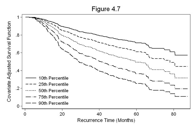
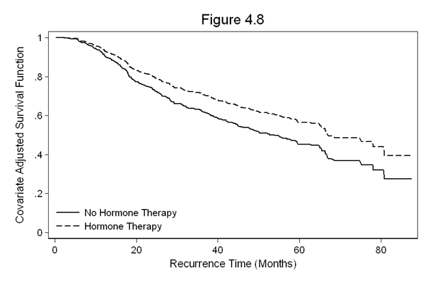
Figure 4.8 on page 129 continuing to use the gbcs dataset.
quietly stcox hormone grade2 grade3 size ln_prg, nohr basesurv(s48)

gen s48_noh = s48^(exp(.35))
gen s48_h = s48^(exp(.35-.326))

sort months
twoway line s48_noh s48_h months, ///
   legend(row(2) col(1) pos(7) order(1 "No Hormone Therapy"  2 "Hormone Therapy") ///
   ring(0) size(medsmall))  ///
   ylabel(0(0.2)1) ///
   xtitle(Recurrence Time (Months)) ///
   ytitle(Covariate Adjusted Survival Function) ///
   title(Figure 4.8)