Table 5.1 on page 142 using the whas500 data. For each variable, we run separate tests. The numbers seen in the table have been italicized in the output shown here.
use https://stats.idre.ucla.edu/stat/examples/asa2/whas500, clear

generate time = lenfol/365.25
stset time, fail(fstat)

stci, p(50) by(gender)

         failure _d:  fstat
   analysis time _t:  time

             |    no. of
gender       |  subjects         50%     Std. Err.     [95% Conf. Interval]
-------------+-------------------------------------------------------------
           0 |       300    5.913758             .      4.44627          .
           1 |       200    3.605749      .3012859      2.36824    4.32307
-------------+-------------------------------------------------------------
       total |       500    4.454483      .4368392       4.1232    6.44216
sts test gender

         failure _d:  fstat
   analysis time _t:  time


Log-rank test for equality of survivor functions

       |   Events         Events
gender |  observed       expected
-------+-------------------------
0      |       111         130.73
1      |       104          84.27
-------+-------------------------
Total  |       215         215.00

             chi2(1) =       7.79
             Pr>chi2 =     0.0053


stci, p(50) by(cvd)

         failure _d:  fstat
   analysis time _t:  time

             |    no. of
cvd          |  subjects         50%     Std. Err.     [95% Conf. Interval]
-------------+-------------------------------------------------------------
           0 |       125    6.442163       .091912      4.31485          .
           1 |       375    4.317591      .4139239      3.72074    6.43395
-------------+-------------------------------------------------------------
       total |       500    4.454483      .4368392       4.1232    6.44216
sts test cvd

         failure _d:  fstat
   analysis time _t:  time


Log-rank test for equality of survivor functions

      |   Events         Events
cvd   |  observed       expected
------+-------------------------
0     |        45          55.84
1     |       170         159.16
------+-------------------------
Total |       215         215.00

            chi2(1) =       2.86
            Pr>chi2 =     0.0907


stci, p(50) by(afb)

         failure _d:  fstat
   analysis time _t:  time

             |    no. of
afb          |  subjects         50%     Std. Err.     [95% Conf. Interval]
-------------+-------------------------------------------------------------
           0 |       422    5.913758      .3102473      4.31485          .
           1 |        78    2.368241        .28552      1.14716    3.77002
-------------+-------------------------------------------------------------
       total |       500    4.454483      .4368392       4.1232    6.44216
sts test afb

         failure _d:  fstat
   analysis time _t:  time


Log-rank test for equality of survivor functions

      |   Events         Events
afb   |  observed       expected
------+-------------------------
0     |       168         184.77
1     |        47          30.23
------+-------------------------
Total |       215         215.00

            chi2(1) =      10.90
            Pr>chi2 =     0.0010


stci, p(50) by(sho)

         failure _d:  fstat
   analysis time _t:  time

             |    no. of
sho          |  subjects         50%     Std. Err.     [95% Conf. Interval]
-------------+-------------------------------------------------------------
           0 |       478    5.273101      .4557953      4.20534          .
           1 |        22    .0465435      .0029195      .010951    1.22108
-------------+-------------------------------------------------------------
       total |       500    4.454483      .4368392       4.1232    6.44216
sts test sho

         failure _d:  fstat
   analysis time _t:  time


Log-rank test for equality of survivor functions

      |   Events         Events
sho   |  observed       expected
------+-------------------------
0     |       198         209.33
1     |        17           5.67
------+-------------------------
Total |       215         215.00

            chi2(1) =      23.84
            Pr>chi2 =     0.0000

stci, p(50) by(chf)

         failure _d:  fstat
   analysis time _t:  time

             |    no. of
chf          |  subjects         50%     Std. Err.     [95% Conf. Interval]
-------------+-------------------------------------------------------------
           0 |       345    6.455852       .112291      5.91376          .
           1 |       155    .9828885      .1189753      .709103    1.53867
-------------+-------------------------------------------------------------
       total |       500    4.454483      .4368392       4.1232    6.44216

sts test chf

         failure _d:  fstat
   analysis time _t:  time


Log-rank test for equality of survivor functions

      |   Events         Events
chf   |  observed       expected
------+-------------------------
0     |       105         162.38
1     |       110          52.62
------+-------------------------
Total |       215         215.00

            chi2(1) =      84.60
            Pr>chi2 =     0.0000

stci, p(50) by(av3)

         failure _d:  fstat
   analysis time _t:  time

             |    no. of
av3          |  subjects         50%     Std. Err.     [95% Conf. Interval]
-------------+-------------------------------------------------------------
           0 |       489    4.454483       .444643       4.1232          .
           1 |        11    5.349761      .5643151      .005476          .
-------------+-------------------------------------------------------------
       total |       500    4.454483      .4368392       4.1232    6.44216
sts test av3

         failure _d:  fstat
   analysis time _t:  time


Log-rank test for equality of survivor functions

      |   Events         Events
av3   |  observed       expected
------+-------------------------
0     |       208         210.54
1     |         7           4.46
------+-------------------------
Total |       215         215.00

            chi2(1) =       1.52
            Pr>chi2 =     0.2171

stci, p(50) by(miord)

         failure _d:  fstat
   analysis time _t:  time

             |    no. of
miord        |  subjects         50%     Std. Err.     [95% Conf. Interval]
-------------+-------------------------------------------------------------
           0 |       329    5.913758      .1091955       5.2731    6.44216
           1 |       171    3.373032      .2971829      1.96578    4.31759
-------------+-------------------------------------------------------------
       total |       500    4.454483      .4368392       4.1232    6.44216
sts test miord

         failure _d:  fstat
   analysis time _t:  time


Log-rank test for equality of survivor functions

      |   Events         Events
miord |  observed       expected
------+-------------------------
0     |       125         146.06
1     |        90          68.94
------+-------------------------
Total |       215         215.00

            chi2(1) =       9.57
            Pr>chi2 =     0.0020

stci , p(50) by(mitype)

         failure _d:  fstat
   analysis time _t:  time

             |    no. of
mitype       |  subjects         50%     Std. Err.     [95% Conf. Interval]
-------------+-------------------------------------------------------------
           0 |       347    3.501711      .3220688      2.60917    4.44627
           1 |       153    6.433949      .1684645      6.43395          .
-------------+-------------------------------------------------------------
       total |       500    4.454483      .4368392       4.1232    6.44216
sts test mitype

         failure _d:  fstat
   analysis time _t:  time


Log-rank test for equality of survivor functions

       |   Events         Events
mitype |  observed       expected
-------+-------------------------
0      |       169         141.21
1      |        46          73.79
-------+-------------------------
Total  |       215         215.00

             chi2(1) =      16.18
             Pr>chi2 =     0.0001
Table 5.2 on page 143 using the whas500 data. We are running the Cox regressions using the quietly command, and then displaying the output from the lincom that corresponds to the table in the text.
quietly stcox age, nohr nolog
lincom 5*age, hr

 ( 1)  5 age = 0

------------------------------------------------------------------------------
          _t | Haz. Ratio   Std. Err.      z    P>|z|     [95% Conf. Interval]
-------------+----------------------------------------------------------------
         (1) |   1.392687   .0423237    10.90   0.000     1.312157     1.47816
------------------------------------------------------------------------------

quietly stcox hr, nohr nolog
lincom 10*hr, hr

 ( 1)  10 hr = 0

------------------------------------------------------------------------------
          _t | Haz. Ratio   Std. Err.      z    P>|z|     [95% Conf. Interval]
-------------+----------------------------------------------------------------
         (1) |   1.162248   .0312287     5.60   0.000     1.102625    1.225095
------------------------------------------------------------------------------

quietly stcox sysbp, nohr nolog
lincom 10*sysbp, hr

 ( 1)  10 sysbp = 0

------------------------------------------------------------------------------
          _t | Haz. Ratio   Std. Err.      z    P>|z|     [95% Conf. Interval]
-------------+----------------------------------------------------------------
         (1) |   .9559761   .0212814    -2.02   0.043     .9151622    .9986101
------------------------------------------------------------------------------

quietly stcox diasbp, nohr nolog
lincom 10*diasbp, hr

 ( 1)  10 diasbp = 0

------------------------------------------------------------------------------
          _t | Haz. Ratio   Std. Err.      z    P>|z|     [95% Conf. Interval]
-------------+----------------------------------------------------------------
         (1) |   .8522054   .0279873    -4.87   0.000     .7990794    .9088635
------------------------------------------------------------------------------

quietly stcox bmi, nohr nolog
lincom 5*bmi, hr

 ( 1)  5 bmi = 0

------------------------------------------------------------------------------
          _t | Haz. Ratio   Std. Err.      z    P>|z|     [95% Conf. Interval]
-------------+----------------------------------------------------------------
         (1) |   .6118107      .0451    -6.67   0.000     .5295051    .7069096
------------------------------------------------------------------------------
Table 5.3 on page 143 using the whas500 data in a multivariate model.
stcox age hr sysbp diasbp bmi gender cvd afb chf miord mitype, nolog nohr

         failure _d:  fstat
   analysis time _t:  time

Cox regression -- Breslow method for ties

No. of subjects =          500                     Number of obs   =       500
No. of failures =          215
Time at risk    =  1207.989046
                                                   LR chi2(11)     =    208.77
Log likelihood  =   -1123.1942                     Prob > chi2     =    0.0000

------------------------------------------------------------------------------
          _t |      Coef.   Std. Err.      z    P>|z|     [95% Conf. Interval]
-------------+----------------------------------------------------------------
         age |   .0486034   .0068246     7.12   0.000     .0352274    .0619795
          hr |   .0104108   .0030766     3.38   0.001     .0043807    .0164408
       sysbp |   .0003598   .0029925     0.12   0.904    -.0055054     .006225
      diasbp |  -.0105894   .0049118    -2.16   0.031    -.0202164   -.0009624
         bmi |  -.0437268   .0164443    -2.66   0.008     -.075957   -.0114966
      gender |  -.2705711   .1457033    -1.86   0.063    -.5561443    .0150021
         cvd |   .0073416   .1781041     0.04   0.967     -.341736    .3564193
         afb |   .1280092   .1711795     0.75   0.455    -.2074965    .4635149
         chf |   .7735398    .149917     5.16   0.000     .4797079    1.067372
       miord |   .0438507   .1484028     0.30   0.768    -.2470134    .3347149
      mitype |  -.1641189   .1878532    -0.87   0.382    -.5323045    .2040666
------------------------------------------------------------------------------
Table 5.4 on page 144 using the whas500 data in a multivariate model.
stcox age hr diasbp bmi gender afb chf miord mitype, nolog nohr

         failure _d:  fstat
   analysis time _t:  time

Cox regression -- Breslow method for ties

No. of subjects =          500                     Number of obs   =       500
No. of failures =          215
Time at risk    =  1207.989046
                                                   LR chi2(9)      =    208.75
Log likelihood  =   -1123.2029                     Prob > chi2     =    0.0000

------------------------------------------------------------------------------
          _t |      Coef.   Std. Err.      z    P>|z|     [95% Conf. Interval]
-------------+----------------------------------------------------------------
         age |   .0487438   .0067402     7.23   0.000     .0355332    .0619544
          hr |   .0103141   .0029871     3.45   0.001     .0044595    .0161687
      diasbp |  -.0101573   .0035359    -2.87   0.004    -.0170876   -.0032269
         bmi |  -.0435961   .0163254    -2.67   0.008    -.0755934   -.0115988
      gender |  -.2682873   .1446723    -1.85   0.064    -.5518399    .0152653
         afb |   .1254387   .1697283     0.74   0.460    -.2072226       .4581
         chf |   .7758481   .1486089     5.22   0.000       .48458    1.067116
       miord |    .044752   .1453871     0.31   0.758    -.2402015    .3297055
      mitype |  -.1691959   .1837834    -0.92   0.357    -.5294048     .191013
------------------------------------------------------------------------------
Table 5.5 on page 144 using the whas500 data in a multivariate model.
stcox age hr diasbp bmi gender afb chf mitype, nolog nohr

         failure _d:  fstat
   analysis time _t:  time

Cox regression -- Breslow method for ties

No. of subjects =          500                     Number of obs   =       500
No. of failures =          215
Time at risk    =  1207.989046
                                                   LR chi2(8)      =    208.66
Log likelihood  =   -1123.2502                     Prob > chi2     =    0.0000

------------------------------------------------------------------------------
          _t |      Coef.   Std. Err.      z    P>|z|     [95% Conf. Interval]
-------------+----------------------------------------------------------------
         age |   .0486987   .0067245     7.24   0.000     .0355188    .0618785
          hr |   .0103887   .0029796     3.49   0.000     .0045487    .0162286
      diasbp |  -.0102109   .0035346    -2.89   0.004    -.0171386   -.0032832
         bmi |  -.0439615   .0162951    -2.70   0.007    -.0758994   -.0120236
      gender |  -.2735672   .1437035    -1.90   0.057    -.5552208    .0080865
         afb |   .1243358   .1697183     0.73   0.464    -.2083059    .4569776
         chf |   .7773988   .1486096     5.23   0.000     .4861293    1.068668
      mitype |  -.1820374   .1789234    -1.02   0.309    -.5327207     .168646
------------------------------------------------------------------------------
Table 5.6 on page 145 using the whas500 data in a multivariate model.
stcox age hr diasbp bmi gender chf, nolog nohr

         failure _d:  fstat
   analysis time _t:  time

Cox regression -- Breslow method for ties

No. of subjects =          500                     Number of obs   =       500
No. of failures =          215
Time at risk    =  1207.989046
                                                   LR chi2(6)      =    207.16
Log likelihood  =   -1123.9997                     Prob > chi2     =    0.0000

------------------------------------------------------------------------------
          _t |      Coef.   Std. Err.      z    P>|z|     [95% Conf. Interval]
-------------+----------------------------------------------------------------
         age |   .0497904    .006596     7.55   0.000     .0368625    .0627184
          hr |   .0111788   .0029156     3.83   0.000     .0054644    .0168933
      diasbp |  -.0105912   .0035124    -3.02   0.003    -.0174753   -.0037071
         bmi |  -.0451558   .0162751    -2.77   0.006    -.0770543   -.0132573
      gender |  -.2699895   .1436178    -1.88   0.060    -.5514751    .0114962
         chf |    .777637   .1466956     5.30   0.000     .4901189    1.065155
------------------------------------------------------------------------------
Table 5.7 on page 146 continuing to use the whas500 data.
summarize age, detail

                             age
-------------------------------------------------------------
      Percentiles      Smallest
 1%         35.5             30
 5%           46             32
10%           49             32       Obs                 500
25%           59             33       Sum of Wgt.         500

50%           72                      Mean             69.846
                        Largest       Std. Dev.      14.49146
75%           82             97
90%           87             98       Variance       210.0023
95%           90            102       Skewness      -.3794081
99%           95            104       Kurtosis       2.372922

/* Calculating Quartile Midpoints for Age */
display (r(min)+r(p25))/2
44.5

display (r(p25)+1+r(p50))/2
66

display (r(p50)+1+r(p75))/2
77.5

display (r(p75)+1+r(max))/2
93.5

gen age_q=age
recode age_q 30/59=1 60/72=2 73/82=3 83/104=4

/* Calculating Coefficients for Age */
xi: stcox i.age_q hr diasbp bmi gender chf, nolog nohr

i.age_q           _Iage_q_1-4         (naturally coded; _Iage_q_1 omitted)

         failure _d:  fstat
   analysis time _t:  time

Cox regression -- Breslow method for ties

No. of subjects =          500                     Number of obs   =       500
No. of failures =          215
Time at risk    =  1207.989046
                                                   LR chi2(8)      =    205.02
Log likelihood  =   -1125.0675                     Prob > chi2     =    0.0000

------------------------------------------------------------------------------
          _t |      Coef.   Std. Err.      z    P>|z|     [95% Conf. Interval]
-------------+----------------------------------------------------------------
   _Iage_q_2 |    .689723   .2944466     2.34   0.019     .1126183    1.266828
   _Iage_q_3 |   1.428489    .273315     5.23   0.000     .8928017    1.964177
   _Iage_q_4 |   1.807118   .2781617     6.50   0.000     1.261931    2.352305
          hr |   .0099286   .0029392     3.38   0.001     .0041679    .0156892
      diasbp |  -.0112784   .0034908    -3.23   0.001    -.0181203   -.0044364
         bmi |  -.0493604   .0162702    -3.03   0.002    -.0812493   -.0174714
      gender |  -.2991236    .144762    -2.07   0.039    -.5828519   -.0153953
         chf |    .833958   .1460775     5.71   0.000     .5476515    1.120265
------------------------------------------------------------------------------

summarize hr, detail

                             hr
-------------------------------------------------------------
      Percentiles      Smallest
 1%           42             35
 5%           54             36
10%           59             36       Obs                 500
25%           69             38       Sum of Wgt.         500

50%           85                      Mean             87.018
                        Largest       Std. Dev.      23.58623
75%        100.5            154
90%          117            157       Variance       556.3103
95%        128.5            160       Skewness       .5650649
99%          150            186       Kurtosis       3.455084

/* Calculating Quartile Midpoints for HR */
display (r(min)+r(p25))/2
52

display (r(p25)+1+r(p50))/2
77.5

display (r(p50)-0.5+r(p75))/2
92.5

display (r(p75)+0.5+r(max))/2
143.5

gen hr_q=hr
recode hr_q 35/69=1 70/85=2 86/100.5=3 100.6/186=4

/* Calculating Coefficients for HR */
xi: stcox age i.hr_q diasbp bmi gender chf, nolog nohr

i.hr_q            _Ihr_q_1-4          (naturally coded; _Ihr_q_1 omitted)

         failure _d:  fstat
   analysis time _t:  time

Cox regression -- Breslow method for ties

No. of subjects =          500                     Number of obs   =       500
No. of failures =          215
Time at risk    =  1207.989046
                                                   LR chi2(8)      =    209.47
Log likelihood  =   -1122.8425                     Prob > chi2     =    0.0000

------------------------------------------------------------------------------
          _t |      Coef.   Std. Err.      z    P>|z|     [95% Conf. Interval]
-------------+----------------------------------------------------------------
         age |   .0504863   .0066777     7.56   0.000     .0373982    .0635744
    _Ihr_q_2 |    .334802   .2370135     1.41   0.158     -.129736      .79934
    _Ihr_q_3 |   .4828416   .2122658     2.27   0.023     .0668082     .898875
    _Ihr_q_4 |     .80903   .2078297     3.89   0.000     .4016912    1.216369
      diasbp |  -.0100241   .0035105    -2.86   0.004    -.0169046   -.0031436
         bmi |  -.0458672   .0162975    -2.81   0.005    -.0778097   -.0139247
      gender |  -.2691365   .1439823    -1.87   0.062    -.5513366    .0130637
         chf |   .7502223   .1487723     5.04   0.000     .4586339    1.041811
------------------------------------------------------------------------------

summarize diasbp, detail

                           diasbp
-------------------------------------------------------------
      Percentiles      Smallest
 1%           26              6
 5%           48             11
10%           52             20       Obs                 500
25%           63             21       Sum o
f Wgt.         500

50%           79                      Mean             78.266
                        Largest       Std. Dev.      21.54529
75%         91.5            138
90%          103            140       Variance       464.1996
95%          110            150       Skewness       .3069473
99%          134            198       Kurtosis       4.978975

/* Calculating Quartile Midpoints for diasbp */
display (r(min)+r(p25))/2
34.5

display (r(p25)+1+r(p50))/2
71.5

display (r(p50)+1+r(p75))/2
85.75

display (r(p75)+1+r(max))/2
145.25

gen diasbp_q=diasbp
recode diasbp_q 6/63=1 64/79=2 80/91=3 92/198=4

/* Calculating Coefficients for diasbp */
xi: stcox age hr i.diasbp_q bmi gender chf, nolog nohr

i.diasbp_q        _Idiasbp_q_1-4      (naturally coded; _Idiasbp_q_1 omitted)

         failure _d:  fstat
   analysis time _t:  time

Cox regression -- Breslow method for ties

No. of subjects =          500                     Number of obs   =       500
No. of failures =          215
Time at risk    =  1207.989046
                                                   LR chi2(8)      =    206.50
Log likelihood  =   -1124.3303                     Prob > chi2     =    0.0000

------------------------------------------------------------------------------
          _t |      Coef.   Std. Err.      z    P>|z|     [95% Conf. Interval]
-------------+----------------------------------------------------------------
         age |   .0499355    .006599     7.57   0.000     .0370018    .0628692
          hr |    .011136   .0029239     3.81   0.000     .0054052    .0168668
_Idiasbp_q_2 |  -.3136974   .1769299    -1.77   0.076    -.6604736    .0330787
_Idiasbp_q_3 |  -.2980701   .2113169    -1.41   0.158    -.7122437    .1161035
_Idiasbp_q_4 |  -.6104616   .2125098    -2.87   0.004    -1.026973     -.19395
         bmi |  -.0458759   .0164737    -2.78   0.005    -.0781637   -.0135882
      gender |  -.2525157   .1442736    -1.75   0.080    -.5352866    .0302553
         chf |   .7687909   .1505416     5.11   0.000     .4737349    1.063847
------------------------------------------------------------------------------

summarize bmi, detail

                             bmi
-------------------------------------------------------------
      Percentiles      Smallest
 1%     15.42587       13.04546
 5%     18.60004       14.59031
10%     20.07724       14.83911       Obs                 500
25%      23.2068       14.84283       Sum of Wgt.         500

50%     25.94592                      Mean           26.61378
                        Largest       Std. Dev.      5.405655
75%     29.39656       42.13576
90%     34.16071       42.38277       Variance       29.22111
95%     36.86193       42.76594       Skewness        .528979
99%     40.89478       44.83886       Kurtosis       3.391798

/* Calculating Quartile Midpoints for bmi */
display (r(min)+r(p25))/2
18.12613

display (r(p25)+r(p50))/2
24.576362

display (r(p50)+r(p75))/2
27.671245

display (r(p75)+r(max))/2
37.117712

generate bmi_q=bmi
recode bmi_q 13/23=1 23/26=2 26/29=3 29/45=4

/* Calculating Coefficients for bmi */
xi: stcox age hr diasbp i.bmi_q gender chf, nolog nohr

i.bmi_q           _Ibmi_q_1-4         (naturally coded; _Ibmi_q_1 omitted)

         failure _d:  fstat
   analysis time _t:  time

Cox regression -- Breslow method for ties

No. of subjects =          500                     Number of obs   =       500
No. of failures =          215
Time at risk    =  1207.989046
                                                   LR chi2(8)      =    209.19
Log likelihood  =   -1122.9827                     Prob > chi2     =    0.0000

------------------------------------------------------------------------------
          _t |      Coef.   Std. Err.      z    P>|z|     [95% Conf. Interval]
-------------+----------------------------------------------------------------
         age |   .0502594   .0066119     7.60   0.000     .0373004    .0632185
          hr |   .0114025   .0029193     3.91   0.000     .0056809    .0171241
      diasbp |  -.0111158   .0035745    -3.11   0.002    -.0181217     -.00411
   _Ibmi_q_2 |    -.45295   .1755822    -2.58   0.010    -.7970849   -.1088152
   _Ibmi_q_3 |  -.3151134   .1925495    -1.64   0.102    -.6925034    .0622767
   _Ibmi_q_4 |  -.5921103   .2224768    -2.66   0.008    -1.028157   -.1560638
      gender |  -.2520627   .1429792    -1.76   0.078    -.5322968    .0281714
         chf |   .7763868   .1460653     5.32   0.000     .4901041    1.062669
------------------------------------------------------------------------------
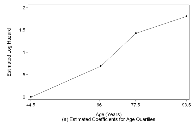
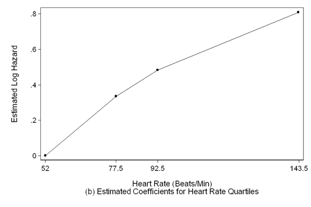
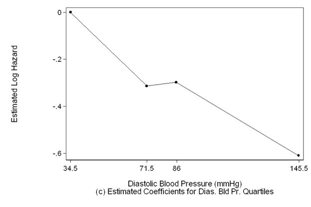
Figure 5.1 on page 146 using the results from Table 5.7.
clear
input agemp age_coeff hrmp hr_coeff diasmp dias_coeff bmimp bmi_coeff
44.55 0.000 52 0.000 34.5 0.000 18.1 0.000
66.5 0.6900 77.5 0.335 71.5 -0.314 24.6 -0.453
77.58 1.428 92.5 0.483 85.8 -0.298 27.7 -0.315
93.5 1.807 143.25 0.809 145.3 -0.610 37.1 -0.592
end
list, clean
agemp age_co~f hrmp hr_coeff diasmp dias_c~f bmimp bmi_co~f
1. 44.55 0 52 0 34.5 0 18.1 0
2. 66.5 .69 77.5 .335 71.5 -.314 24.6 -.453
3. 77.58 1.428 92.5 .483 85.8 -.298 27.7 -.315
4. 93.5 1.807 143.25 .809 145.3 -.61 37.1 -.592
label variable agemp "Age (Years)"
label variable hrmp "Hear Rate (Beats/Min)"
label variable diasmp "Diastolic Blood pressure (mmHg)"
label variable bmimp "Body mass Index (kg/m^2)"
scatter age_coeff agemp if agemp>=44.5 & agemp<=93.5, sort ms(o) c(l) mc(black) ///
clpattern(solid) lc(black) ylabel(,nogrid) clwidth(thin) ///
ytitle(Estimated Log Hazard) yscale(titlegap(3)) xlabel(44.5 66 77.5 93.5) ///
xscale(titlegap(3) ) lc(black) graphregion(fcolor(white)) ///
xtitle("Age (Years)" "(a) Estimated Coefficients for Age Quartiles")
 scatter hr_coeff hrmp if hrmp>=52 &hrmp<=143.5, sort ms(o) c(l) clpattern(solid) ///
lc(black) mc(black) ylabel(,nogrid) clwidth(thin) ///
ytitle(Estimated Log Hazard) yscale(titlegap(3)) xlabel(52 77.5 92.5 143.5) ///
xscale(titlegap(3) ) lc(black) graphregion(fcolor(white)) ///
xtitle("Heart Rate (Beats/Min)" "(b) Estimated Coefficients for Heart Rate Quartiles")
scatter hr_coeff hrmp if hrmp>=52 &hrmp<=143.5, sort ms(o) c(l) clpattern(solid) ///
lc(black) mc(black) ylabel(,nogrid) clwidth(thin) ///
ytitle(Estimated Log Hazard) yscale(titlegap(3)) xlabel(52 77.5 92.5 143.5) ///
xscale(titlegap(3) ) lc(black) graphregion(fcolor(white)) ///
xtitle("Heart Rate (Beats/Min)" "(b) Estimated Coefficients for Heart Rate Quartiles")
 scatter dias_coeff diasmp if diasmp>=34.5 &diasmp<=145.5, sort ms(o) c(l) clpattern(solid) ///
lc(black) mc(black) ylabel(,nogrid) clwidth(thin) ///
ytitle(Estimated Log Hazard) yscale(titlegap(3)) xlabel(34.5 71.5 86 145.5) ///
xscale(titlegap(3) ) lc(black) graphregion(fcolor(white)) ///
xtitle("Diastolic Blood Pressure (mmHg)" "(c) Estimated Coefficients for Dias. Bld Pr. Quartiles")
scatter dias_coeff diasmp if diasmp>=34.5 &diasmp<=145.5, sort ms(o) c(l) clpattern(solid) ///
lc(black) mc(black) ylabel(,nogrid) clwidth(thin) ///
ytitle(Estimated Log Hazard) yscale(titlegap(3)) xlabel(34.5 71.5 86 145.5) ///
xscale(titlegap(3) ) lc(black) graphregion(fcolor(white)) ///
xtitle("Diastolic Blood Pressure (mmHg)" "(c) Estimated Coefficients for Dias. Bld Pr. Quartiles")
 scatter bmi_coeff bmimp if bmimp>=18.1 &bmimp<=37.1, sort ms(o) c(l) clpattern(solid) lc(black) ///
mc(black) ylabel(,nogrid) clwidth(thin) ///
ytitle(Estimated Log Hazard) yscale(titlegap(3)) xlabel(18.1 24.6 27.7 37.1) ///
xscale(titlegap(3) ) lc(black) graphregion(fcolor(white)) ///
xtitle("Body Mass Index (kg/m^2)" "(d) Estimated Coefficients for Body Mass Index Quartiles")
scatter bmi_coeff bmimp if bmimp>=18.1 &bmimp<=37.1, sort ms(o) c(l) clpattern(solid) lc(black) ///
mc(black) ylabel(,nogrid) clwidth(thin) ///
ytitle(Estimated Log Hazard) yscale(titlegap(3)) xlabel(18.1 24.6 27.7 37.1) ///
xscale(titlegap(3) ) lc(black) graphregion(fcolor(white)) ///
xtitle("Body Mass Index (kg/m^2)" "(d) Estimated Coefficients for Body Mass Index Quartiles")
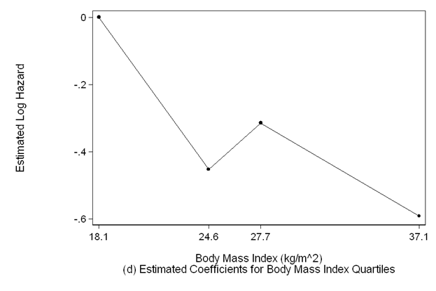
Table 5.8 on page 147 using the whas500 data.
use https://stats.idre.ucla.edu/stat/examples/asa2/whas500, clear

generate time = lenfol/365.25
stset time, fail(fstat)

fracpoly stcox bmi age hr diasbp gender chf, nolog nohr comp log

-> gen double Iage__1 = age-69.846 if e(sample)
-> gen double Ihr__1 = hr-87.018 if e(sample)
-> gen double Idias__1 = diasbp-78.266 if e(sample)

Model #      Deviance  Power 1 Power 2

    1        2241.668    -2.0      .
. . . [additional output omitted for space] . . .
   43        2237.784     3.0     2.0
   44        2237.922     3.0     3.0
-> gen double Ibmi__1 = X^2-7.082932813 if e(sample)
-> gen double Ibmi__2 = X^3-18.8503615 if e(sample)
   (where: X = bmi/10)

         failure _d:  fstat
   analysis time _t:  time

Cox regression -- Breslow method for ties

No. of subjects =          500                     Number of obs   =       500
No. of failures =          215
Time at risk    =  1207.989046
                                                   LR chi2(7)      =    217.37
Log likelihood  =   -1118.8921                     Prob > chi2     =    0.0000

------------------------------------------------------------------------------
          _t |      Coef.   Std. Err.      z    P>|z|     [95% Conf. Interval]
-------------+----------------------------------------------------------------
     Ibmi__1 |  -.7247551    .172612    -4.20   0.000    -1.063068   -.3864418
     Ibmi__2 |   .1544204   .0392284     3.94   0.000     .0775343    .2313066
     Iage__1 |   .0497816   .0066127     7.53   0.000     .0368209    .0627423
      Ihr__1 |   .0118002    .002954     3.99   0.000     .0060105    .0175899
    Idias__1 |  -.0106741   .0035015    -3.05   0.002    -.0175368   -.0038113
      gender |  -.3264025   .1442151    -2.26   0.024     -.609059    -.043746
         chf |     .82341   .1471777     5.59   0.000      .534947    1.111873
------------------------------------------------------------------------------
Deviance:  2237.78. Best powers of bmi among 44 models fit: 2 3.

Fractional polynomial model comparisons:
---------------------------------------------------------------
bmi              df       Deviance   Dev. dif.  P (*)  Powers
---------------------------------------------------------------
Not in model      0       2255.945    18.160    0.001
Linear            1       2247.999    10.215    0.017  1
m = 1             2       2241.668     3.884    0.143  -2
m = 2             4       2237.784        --       --  2 3
---------------------------------------------------------------
(*) P-value from deviance difference comparing reported model with m = 2 model

/* Comparing linear model to model without bmi */
display 2255.945 - 2247.999
7.946
display chi2tail(1,7.946)
.00481938

/* Comparing m = 1 model to linear model */
display 2247.999 - 2241.668
6.331
display chi2tail(1,6.331)
.01186454

/* Comparing m = 2 model to m = 1 model */
display 2241.668 - 2237.784
3.884
display chi2tail(2,3.884)
.14341683
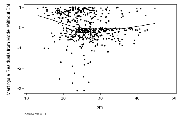
Figure 5.2 on page 149 using the whas500 data.
quietly stcox age hr diasbp gender chf, nolog nohr mgale(M_bmi)

lowess M_bmi bmi, ms(o) ytitle(Martingale Residuals from Model Without BMI) ///
     ylabel(,nogrid angle(horizontal)) lineop(lc(black)) mc(black) ///
     title("")  yscale(titlegap(3)) xscale(titlegap(3)) ///
     graphregion(fcolor(white))


quietly stcox age hr diasbp bmi gender chf, nolog nohr mgale(M_t)

generate Hhat=fstat-M_t
lowess fstat bmi, gen(csm) nograph
lowess Hhat bmi, gen(Hsm) nograph
generate gtfsmooth = ln(csm/Hsm)+_b[bmi]*bmi

twoway line gtfsmooth bmi, sort ytitle("ln(csmoothed/Hsmoothed)+beta*x")
quietly stcox age hr diasbp bmi gender chf, nolog nohr mgale(M_t)
generate Hhat=fstat-M_t
lowess fstat bmi, gen(csm) nograph
lowess Hhat bmi, gen(Hsm) nograph
generate gtfsmooth = ln(csm/Hsm)+_b[bmi]*bmi
twoway line gtfsmooth bmi, sort ytitle("ln(csmoothed/Hsmoothed)+beta*x")
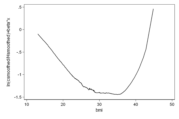
Table 5.9 on page 150 using the whas500 data.
gen bmifp1=(bmi/10)^2
gen bmifp2=(bmi/10)^3

stcox bmifp1 bmifp2 age hr diasbp gender chf, nolog nohr

         failure _d:  fstat
   analysis time _t:  time

Cox regression -- Breslow method for ties

No. of subjects =          500                     Number of obs   =       500
No. of failures =          215
Time at risk    =  1207.989046
                                                   LR chi2(7)      =    217.37
Log likelihood  =   -1118.8921                     Prob > chi2     =    0.0000

------------------------------------------------------------------------------
          _t |      Coef.   Std. Err.      z    P>|z|     [95% Conf. Interval]
-------------+----------------------------------------------------------------
      bmifp1 |  -.7247552    .172612    -4.20   0.000    -1.063068   -.3864419
      bmifp2 |   .1544204   .0392284     3.94   0.000     .0775343    .2313066
         age |   .0497816   .0066127     7.53   0.000     .0368209    .0627423
          hr |   .0118002    .002954     3.99   0.000     .0060105    .0175899
      diasbp |  -.0106741   .0035015    -3.05   0.002    -.0175368   -.0038113
      gender |  -.3264025   .1442151    -2.26   0.024     -.609059    -.043746
         chf |     .82341   .1471777     5.59   0.000      .534947    1.111873
------------------------------------------------------------------------------

est store maineffects
Figure 5.3 on page 150 using the results from the model above on the whas500 data.
gen fp_funct=_b[bmifp1]*bmifp1+_b[bmifp2]*bmifp2
gen diff=gtfsmooth-fp_funct
quietly summarize diff
replace fp_funct=fp_funct+r(mean)

line gtfsmooth fp_funct bmi, sort clpattern(solid shortdash) ///
      legend(row(2) col(1) order(1 "GTF Smooth" 2 "Two Term (2, 3) Model") ring(0) ///
      size(medsmall) pos(11) region(lc(white))) ytitle(Estimated Log Hazard) ///
      ylabel(,nogrid angle(horizontal)) yscale(titlegap(3)) ///
      xscale(titlegap(3)) lc(black black) graphregion(fcolor(white))
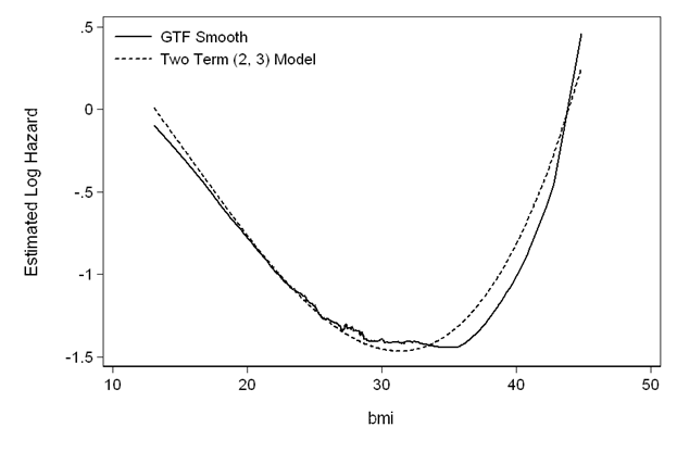
Table 5.10 on page 151 using the whas500 data. Since the BMI test requires removing two variables, we will do these first and then examine the rest of the variables using a foreach loop.
gen bmiage1 = age * bmifp1
gen bmiage2 = age * bmifp2
quietly stcox bmifp1 bmifp2 age hr diasbp gender chf bmiage1 bmiage2, nolog nohr
est store A
quietly stcox bmifp1 bmifp2 age hr diasbp gender chf, nolog nohr
lrtest A

Likelihood-ratio test                                  LR chi2(2)  =      3.32
(Assumption: . nested in A)                            Prob > chi2 =    0.1899

foreach varname of varlist hr diasbp gender chf {
     capture drop i1
     gen i1=age*(`varname')
     quietly stcox bmifp1 bmifp2 age hr diasbp gender chf i1, nolog nohr
     est store A
     quietly stcox bmifp1 bmifp2 age hr diasbp gender chf, nolog nohr
     lrtest A
   }

Likelihood-ratio test                                  LR chi2(1)  =      2.27
(Assumption: . nested in A)                            Prob > chi2 =    0.1316

Likelihood-ratio test                                  LR chi2(1)  =      2.70
(Assumption: . nested in A)                            Prob > chi2 =    0.1001

Likelihood-ratio test                                  LR chi2(1)  =      5.23
(Assumption: . nested in A)                            Prob > chi2 =    0.0223

Likelihood-ratio test                                  LR chi2(1)  =      4.99
(Assumption: . nested in A)                            Prob > chi2 =    0.0254

gen bmigender1 = gender * bmifp1
gen bmigender2 = gender * bmifp2
quietly stcox bmifp1 bmifp2 age hr diasbp gender chf bmigender1 bmigender2, nolog nohr
est store A
quietly stcox bmifp1 bmifp2 age hr diasbp gender chf, nolog nohr
lrtest A

Likelihood-ratio test                                  LR chi2(2)  =      3.83
(Assumption: . nested in A)                            Prob > chi2 =    0.1474

foreach varname of varlist hr diasbp chf {
     capture drop i1
     gen i1=gender*(`varname')
     quietly stcox bmifp1 bmifp2 age hr diasbp gender chf i1, nolog nohr
     est store A
     quietly stcox bmifp1 bmifp2 age hr diasbp gender chf, nolog nohr
     lrtest A
   }

Likelihood-ratio test                                  LR chi2(1)  =      2.13
(Assumption: . nested in A)                            Prob > chi2 =    0.1446

Likelihood-ratio test                                  LR chi2(1)  =      3.07
(Assumption: . nested in A)                            Prob > chi2 =    0.0796

Likelihood-ratio test                                  LR chi2(1)  =      0.50
(Assumption: . nested in A)                            Prob > chi2 =    0.4817
Table 5.11 on page 152 using the whas500 data.
generate axg = age*gender

stcox bmifp1 bmifp2 age hr diasbp gender chf axg, nolog nohr

         failure _d:  fstat
   analysis time _t:  time

Cox regression -- Breslow method for ties

No. of subjects =          500                     Number of obs   =       500
No. of failures =          215
Time at risk    =  1207.989046
                                                   LR chi2(8)      =    222.60
Log likelihood  =   -1116.2793                     Prob > chi2     =    0.0000

------------------------------------------------------------------------------
          _t |      Coef.   Std. Err.      z    P>|z|     [95% Conf. Interval]
-------------+----------------------------------------------------------------
      bmifp1 |  -.6730201   .1735831    -3.88   0.000    -1.013237   -.3328035
      bmifp2 |   .1421257   .0394413     3.60   0.000     .0648222    .2194292
         age |   .0605347   .0083175     7.28   0.000     .0442327    .0768367
          hr |   .0116719   .0029427     3.97   0.000     .0059044    .0174394
      diasbp |  -.0107119   .0034741    -3.08   0.002     -.017521   -.0039027
      gender |   1.855257   .9578425     1.94   0.053    -.0220801    3.732594
         chf |    .823524   .1465418     5.62   0.000     .5363074    1.110741
         axg |  -.0276658   .0120503    -2.30   0.022     -.051284   -.0040476
------------------------------------------------------------------------------
Table 5.12 on page 152 using the whas500 data. Our coefficient for gender does not match the text exactly.
generate axd = age*diasbp
generate axc = age*chf
generate gxd = gender*diasbp
stcox bmifp1 bmifp2 age hr diasbp gender chf axg axc axd gxd, nolog nohr

         failure _d:  fstat
   analysis time _t:  time

Cox regression -- Breslow method for ties

No. of subjects =          500                     Number of obs   =       500
No. of failures =          215
Time at risk    =  1207.989046
                                                   LR chi2(11)     =    229.97
Log likelihood  =   -1112.5953                     Prob > chi2     =    0.0000

------------------------------------------------------------------------------
          _t |      Coef.   Std. Err.      z    P>|z|     [95% Conf. Interval]
-------------+----------------------------------------------------------------
      bmifp1 |  -.6410106   .1753848    -3.65   0.000    -.9847585   -.2972627
      bmifp2 |    .137229   .0400039     3.43   0.001     .0588228    .2156352
         age |   .0338233   .0203215     1.66   0.096    -.0060061    .0736527
          hr |    .011193   .0029711     3.77   0.000     .0053697    .0170164
      diasbp |  -.0526922   .0213007    -2.47   0.013    -.0944408   -.0109435
      gender |   .7476962   1.220066     0.61   0.540    -1.643588    3.138981
         chf |   2.456034    1.00301     2.45   0.014     .4901696    4.421898
         axg |  -.0220185   .0131616    -1.67   0.094    -.0478148    .0037779
         axc |   -.020293   .0127172    -1.60   0.111    -.0452182    .0046323
         axd |   .0004845   .0002649     1.83   0.067    -.0000346    .0010037
         gxd |   .0089871   .0069291     1.30   0.195    -.0045937     .022568
------------------------------------------------------------------------------
Table 5.13 on page 153 using the whas500 data.
stcox bmifp1 bmifp2 age hr diasbp gender chf axg, nolog nohr

         failure _d:  fstat
   analysis time _t:  time

Cox regression -- Breslow method for ties

No. of subjects =          500                     Number of obs   =       500
No. of failures =          215
Time at risk    =  1207.989046
                                                   LR chi2(8)      =    222.60
Log likelihood  =   -1116.2793                     Prob > chi2     =    0.0000

------------------------------------------------------------------------------
          _t |      Coef.   Std. Err.      z    P>|z|     [95% Conf. Interval]
-------------+----------------------------------------------------------------
      bmifp1 |  -.6730201   .1735831    -3.88   0.000    -1.013237   -.3328035
      bmifp2 |   .1421257   .0394413     3.60   0.000     .0648222    .2194292
         age |   .0605347   .0083175     7.28   0.000     .0442327    .0768367
          hr |   .0116719   .0029427     3.97   0.000     .0059044    .0174394
      diasbp |  -.0107119   .0034741    -3.08   0.002     -.017521   -.0039027
      gender |   1.855257   .9578425     1.94   0.053    -.0220801    3.732594
         chf |    .823524   .1465418     5.62   0.000     .5363074    1.110741
         axg |  -.0276658   .0120503    -2.30   0.022     -.051284   -.0040476
------------------------------------------------------------------------------
Table 5.14 on page 158 using the whas500 data.
Stata computes the Wald test but not the score test and the output is not formatted as in the book. However, we can compare the order in which variables were added to that shown in the book. Stata provides the p-values at each step and the final model.
stepwise stcox age chf hr diasbp bmi gender mitype miord sysbp cvd afb, ///
   pe(.25) pr(.8) forward

                      begin with empty model
p = 0.0000 <  0.2500  adding   age
p = 0.0000 <  0.2500  adding   chf
p = 0.0025 <  0.2500  adding   hr
p = 0.0022 <  0.2500  adding   diasbp
p = 0.0074 <  0.2500  adding   bmi
p = 0.0601 <  0.2500  adding   gender

Cox regression -- Breslow method for ties

No. of subjects =          500                     Number of obs   =       500
No. of failures =          215
Time at risk    =  1207.989046
                                                   LR chi2(6)      =    207.16
Log likelihood  =   -1123.9997                     Prob > chi2     =    0.0000

------------------------------------------------------------------------------
          _t | Haz. Ratio   Std. Err.      z    P>|z|     [95% Conf. Interval]
-------------+----------------------------------------------------------------
         age |   1.051051   .0069327     7.55   0.000      1.03755    1.064727
         chf |   2.176323    .319257     5.30   0.000      1.63251    2.901289
          hr |   1.011242   .0029484     3.83   0.000     1.005479    1.017037
      diasbp |   .9894647   .0034754    -3.02   0.003     .9826765    .9962998
         bmi |   .9558485   .0155565    -2.77   0.006     .9258395    .9868302
      gender |   .7633875    .109636    -1.88   0.060     .5760994    1.011563
------------------------------------------------------------------------------
Table 5.15 on page 161 using the whas500 data.
Stata does not have built-in score test or Mallow’s C.
It is possible to compute these values manually using the scoretest_cox command.
We will show the process for the first line in Table 5.15.
To get scoretest_cox type command: search scoretest_cox
/* 11-covariate model */
quietly stcox age gender hr diasbp bmi chf sysbp cvd afb miord mitype
scoretest_cox age gender hr diasbp bmi chf sysbp cvd afb miord mitype

 ( 1)  age = 0
 ( 2)  gender = 0
 ( 3)  hr = 0
 ( 4)  diasbp = 0
 ( 5)  bmi = 0
 ( 6)  chf = 0
 ( 7)  sysbp = 0
 ( 8)  cvd = 0
 ( 9)  afb = 0
 (10)  miord = 0
 (11)  mitype = 0

           chi2( 11) =  208.62
         Prob > chi2 =    0.0000

scalar score0 = r(chi2)

/* Model 1 */
quietly stcox age gender hr diasbp bmi chf
scoretest_cox age gender hr diasbp bmi chf

 ( 1)  age = 0
 ( 2)  gender = 0
 ( 3)  hr = 0
 ( 4)  diasbp = 0
 ( 5)  bmi = 0
 ( 6)  chf = 0

           chi2(  6) =  206.49
         Prob > chi2 =    0.0000

scalar score1 = r(chi2)
display score0 - score1
2.1326329
display (score0 - score1) + (11-2*5)
3.1326329

/* Model 2 */
quietly stcox age gender hr diasbp bmi chf mitype
scoretest_cox age gender hr diasbp bmi chf mitype

 ( 1)  age = 0
 ( 2)  gender = 0
 ( 3)  hr = 0
 ( 4)  diasbp = 0
 ( 5)  bmi = 0
 ( 6)  chf = 0
 ( 7)  mitype = 0

           chi2(  7) =  208.04
         Prob > chi2 =    0.0000

scalar score2 = r(chi2)
display score0 - score2
.58451409
display (score0 - score2) + (11-2*4)
3.5845141

/* Model 3 */
quietly stcox age hr diasbp bmi chf
scoretest_cox age hr diasbp bmi chf

 ( 1)  age = 0
 ( 2)  hr = 0
 ( 3)  diasbp = 0
 ( 4)  bmi = 0
 ( 5)  chf = 0

           chi2(  5) =  202.67
         Prob > chi2 =    0.0000

scalar score3 = r(chi2)
display score0 - score3
5.9477082
display (score0 - score3) + (11-2*6)
4.9477082

/* Model 4 */
quietly stcox age gender hr diasbp bmi chf sysbp
scoretest_cox age gender hr diasbp bmi chf sysbp

 ( 1)  age = 0
 ( 2)  gender = 0
 ( 3)  hr = 0
 ( 4)  diasbp = 0
 ( 5)  bmi = 0
 ( 6)  chf = 0
 ( 7)  sysbp = 0

           chi2(  7) =  206.86
         Prob > chi2 =    0.0000

scalar score4 = r(chi2)
display score0 - score4
1.7659588
display (score0 - score4) + (11-2*4)
4.7659588

/* Model 5 */
quietly stcox age gender hr diasbp bmi chf miord
scoretest_cox age gender hr diasbp bmi chf miord

 ( 1)  age = 0
 ( 2)  gender = 0
 ( 3)  hr = 0
 ( 4)  diasbp = 0
 ( 5)  bmi = 0
 ( 6)  chf = 0
 ( 7)  miord = 0

           chi2(  7) =  206.64
         Prob > chi2 =    0.0000

scalar score5 = r(chi2)
display score0 - score5
1.9869457
display (score0 - score5) + (11-2*4)
4.9869457
Table 5.16 on page 165 using the whas500 data. To install the mfp command, type search mfp. We have displayed only the output that corresponds to the table in the text.
mfp stcox age hr sysbp diasbp bmi gender cvd afb chf miord mitype, ///
   adjust(no) df(4, gender cvd afb chf miord mitype:1) ///
   alpha(0.15) select(0.15)

Deviance for model with all terms untransformed =  2246.388, 500 observations

. . . [additional output omitted for space] . . .

Variable     Model (vs.)   Deviance  Dev diff.   P      Powers   (vs.)
----------------------------------------------------------------------
age          null   FP2    2301.581    67.477  0.000*   .         3 3
             lin.          2237.784     3.680  0.298    1
             Final         2237.784                     1

chf          null   lin.   2268.808    31.023  0.000*   .         1
             Final         2237.784                     1

hr           null   FP2    2253.103    18.116  0.001*   .         -2 -2
             lin.          2237.784     2.797  0.424    1
             Final         2237.784                     1

bmi          null   FP2    2255.945    18.160  0.001*   .         2 3
             lin.          2247.999    10.215  0.017+   1
             FP1           2241.668     3.884  0.143+   -2
             Final         2237.784                     2 3

diasbp       null   FP2    2247.368    12.275  0.015*   .         3 3
             lin.          2237.784     2.691  0.442    1
             Final         2237.784                     1

gender       null   lin.   2242.906     5.122  0.024*   .         1
             Final         2237.784                     1

mitype       null   lin.   2237.784     0.852  0.356    .         1
             Final         2237.784                     .

afb          null   lin.   2237.784     0.234  0.629    .         1
             Final         2237.784                     .

miord        null   lin.   2237.784     0.153  0.695    .         1
             Final         2237.784                     .

sysbp        null   FP2    2237.784     3.095  0.542    .         -.5 -.5
             Final         2237.784                     .

cvd          null   lin.   2237.784     0.052  0.820    .         1
             Final         2237.784                     .


Fractional polynomial fitting algorithm converged after 3 cycles.

. . . [additional output omitted for space] . . .
Tables 5.17 & 5.18 use hypothetical data