Table 6.1 on page 180 using the whas500 data. To generate the score tests and global tests in this table, we will first run a Cox regression with the indicated variables. Then we can indicate the various tests.
use https://stats.idre.ucla.edu/stat/examples/asa2/whas500, clear

generate time = lenfol/365.25

stset time, fail(fstat)

generate bmifp1=(bmi/10)^2
generate bmifp2=(bmi/10)^3
generate ga = gender*age

stcox bmifp1 bmifp2 age hr  diasbp  gender  chf  ga, ///
   nolog nohr mgale(mgale) bases(S0) sch(sch*) sca(sca*) esr(scr*)

         failure _d:  fstat
   analysis time _t:  time

Cox regression -- Breslow method for ties

No. of subjects =          500                     Number of obs   =       500
No. of failures =          215
Time at risk    =  1207.989046
                                                   LR chi2(8)      =    222.60
Log likelihood  =   -1116.2793                     Prob > chi2     =    0.0000

------------------------------------------------------------------------------
          _t |      Coef.   Std. Err.      z    P>|z|     [95% Conf. Interval]
-------------+----------------------------------------------------------------
      bmifp1 |  -.6730201   .1735831    -3.88   0.000    -1.013237   -.3328035
      bmifp2 |   .1421257   .0394413     3.60   0.000     .0648222    .2194292
         age |   .0605347   .0083175     7.28   0.000     .0442327    .0768367
          hr |   .0116719   .0029427     3.97   0.000     .0059044    .0174394
      diasbp |  -.0107119   .0034741    -3.08   0.002     -.017521   -.0039027
      gender |   1.855257   .9578425     1.94   0.053    -.0220801    3.732594
         chf |    .823524   .1465418     5.62   0.000     .5363074    1.110741
          ga |  -.0276658   .0120503    -2.30   0.022     -.051284   -.0040476
------------------------------------------------------------------------------

estat phtest, detail       /* g(t) = t */

      Test of proportional-hazards assumption

      Time:  Time
      ----------------------------------------------------------------
                  |       rho            chi2       df       Prob>chi2
      ------------+---------------------------------------------------
      bmifp1      |      0.08343         1.66        1         0.1979
      bmifp2      |     -0.07232         1.24        1         0.2652
      age         |      0.08347         1.41        1         0.2356
      hr          |      0.01913         0.08        1         0.7765
      diasbp      |      0.00023         0.00        1         0.9972
      gender      |      0.03404         0.23        1         0.6304
      chf         |     -0.04372         0.44        1         0.5068
      ga          |     -0.02981         0.18        1         0.6724
      ------------+---------------------------------------------------
      global test |                      3.65        8         0.8869
      ----------------------------------------------------------------

estat phtest, log detail   /* g(t) = ln(t) */

      Test of proportional-hazards assumption

      Time:  Log(t)
      ----------------------------------------------------------------
                  |       rho            chi2       df       Prob>chi2
      ------------+---------------------------------------------------
      bmifp1      |      0.00699         0.01        1         0.9141
      bmifp2      |      0.00352         0.00        1         0.9567
      age         |      0.14584         4.29        1         0.0382
      hr          |      0.06847         1.03        1         0.3098
      diasbp      |      0.04669         0.53        1         0.4667
      gender      |      0.10119         2.05        1         0.1526
      chf         |      0.03799         0.33        1         0.5640
      ga          |     -0.10549         2.24        1         0.1345
      ------------+---------------------------------------------------
      global test |                      7.47        8         0.4869
      ----------------------------------------------------------------

estat phtest, km detail    /* g(t) = Skm(t) */

      Test of proportional-hazards assumption

      Time:  Kaplan-Meier
      ----------------------------------------------------------------
                  |       rho            chi2       df       Prob>chi2
      ------------+---------------------------------------------------
      bmifp1      |      0.03835         0.35        1         0.5540
      bmifp2      |     -0.02760         0.18        1         0.6706
      age         |      0.12766         3.29        1         0.0697
      hr          |      0.05075         0.57        1         0.4516
      diasbp      |      0.03786         0.35        1         0.5550
      gender      |      0.08120         1.32        1         0.2511
      chf         |      0.01055         0.03        1         0.8727
      ga          |     -0.08196         1.35        1         0.2449
      ------------+---------------------------------------------------
      global test |                      5.10        8         0.7466
      ----------------------------------------------------------------

estat phtest, rank detail  /* g(t) = rank(t) */

      Test of proportional-hazards assumption

      Time:  Rank(t)
      ----------------------------------------------------------------
                  |       rho            chi2       df       Prob>chi2
      ------------+---------------------------------------------------
      bmifp1      |      0.02681         0.17        1         0.6791
      bmifp2      |     -0.01530         0.06        1         0.8136
      age         |      0.13833         3.86        1         0.0493
      hr          |      0.06433         0.91        1         0.3399
      diasbp      |      0.04099         0.41        1         0.5228
      gender      |      0.09077         1.65        1         0.1995
      chf         |      0.01952         0.09        1         0.7669
      ga          |     -0.09258         1.73        1         0.1890
      ------------+---------------------------------------------------
      global test |                      6.36        8         0.6072
      ----------------------------------------------------------------
Figure 6.1 on page 181 continuing to use the whas500 data.
sts gen skm = s generate ln_t=ln(time) /* Figure 6.1a */ lowess sca4 ln_t, name(fig6_1a, replace)/* Figure 6.1b */ lowess sca4 _t, name(fig6_1b, replace)
/* Figure 6.1c */ lowess sca4 skm, name(fig6_1c, replace)
/* Figure 6.1d */ egen rank_t=rank(time) if fstat==1 lowess sca4 rank_t, name(fig6_1d, replace)
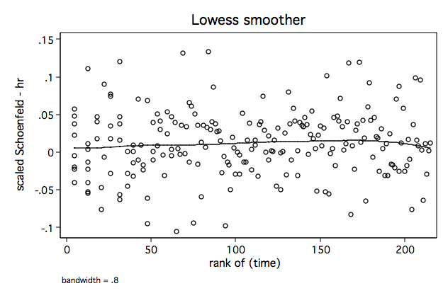
Figure 6.2 on page 182 continuing to use the whas500 data.
/* Figure 6.2a */ lowess sca7 ln_t, name(fig6_2a, replace)/* Figure 6.2b */ lowess sca7 _t, name(fig6_2b, replace)
/* Figure 6.2c */ lowess sca7 skm, name(fig6_2c, replace)
/* Figure 6.2d */ lowess sca7 rank_t, name(fig6_2d, replace)
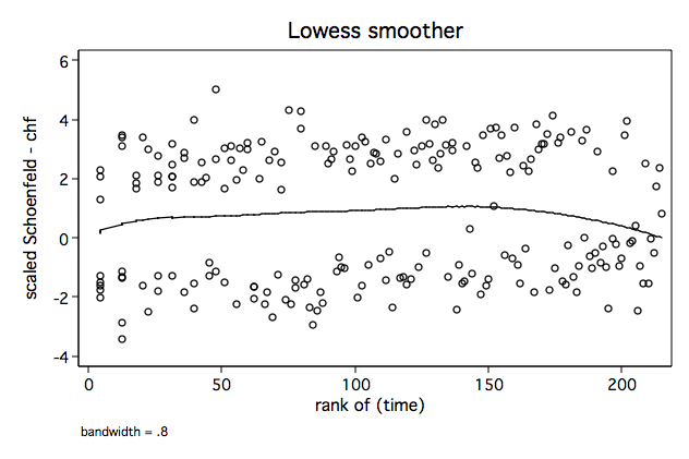
Figure 6.3 on page 183 continuing to use the whas500 data.
/* Figure 6.3a */ lowess sca3 ln_t, name(fig6_3a, replace)/* Figure 6.3b */ lowess sca3 _t, name(fig6_3b, replace)
/* Figure 6.3c */ lowess sca3 skm, name(fig6_3c, replace)
/* Figure 6.3d */ lowess sca3 rank_t, name(fig6_3d, replace)
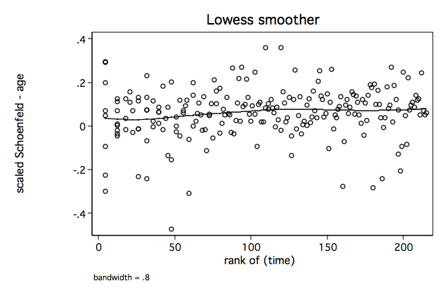
Figure 6.4 on page 186 continuing to use the whas500 data.
/* Figure 6.4a */ twoway scatter scr1 bmi, name(fig6_4a, replace)/* Figure 6.4b */ twoway scatter scr2 bmi, name(fig6_4b, replace)
/* Figure 6.4c */ twoway scatter scr4 hr, name(fig6_4c, replace)
/* Figure 6.4d */ twoway scatter scr5 diasbp, name(fig6_4d, replace)
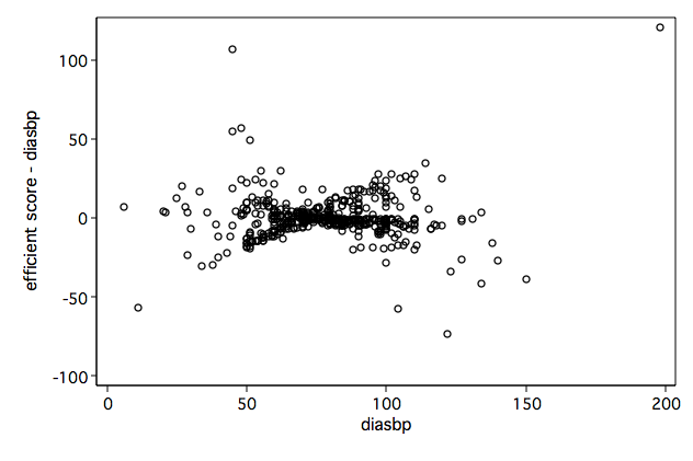
Figure 6.5 on page 186 continuing to use the whas500 data.
/* Figure 6.5a */ twoway scatter scr3 age, name(fig6_5a, replace)/* Figure 6.5b */ twoway scatter scr8 ga if ga~=0, name(fig6_5b, replace) /// ylabel(-200(100)200) xlabel(20(20)100)
/* Figure 6.5c */ graph box scr7, over(chf) name(fig6_5c, replace)
/* Figure 6.5d */ graph box scr6, over(gender) name(fig6_5d, replace)
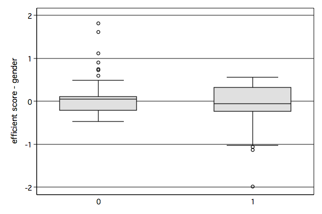
Figure 6.6 on page 187 continuing to use the whas500 data. We will be using the variance-covariance matrix of the estimators from the Cox regression run above.
/* compute scaled score residuals */ set matsize 600 mat V = e(V) mkmat scr1 scr2 scr3 scr4 scr5 scr6 scr7 scr8, mat(L) matrix DB = L*V svmat DB, name(db) /* Figure 6.6a */ twoway scatter db1 bmi, name(fig6_6a, replace)/* Figure 6.6b */ twoway scatter db2 bmi, name(fig6_6b, replace)
/* Figure 6.6c */ twoway scatter db4 hr, name(fig6_6c, replace)
/* Figure 6.6d */ twoway scatter db5 diasbp, name(fig6_6d, replace)
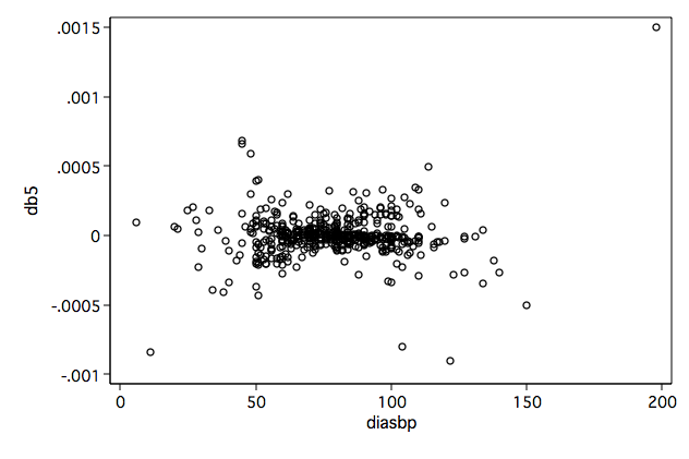
Figure 6.7 on page 188 continuing to use the whas500 data.
/* Figure 6.7a */ twoway scatter db3 age, name(fig6_7a, replace)/* Figure 6.7b */ twoway scatter db8 ga if ga~=0, name(fig6_7b, replace) /// ylabel(-.004(.002).004) xlabel(20(20)100)
/* Figure 6.7c */ graph box db7, over(chf) name(fig6_7c, replace)
/* Figure 6.7d */ graph box db6, over(gender) name(fig6_7d, replace)
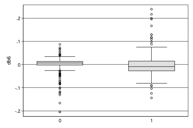
Figure 6.8 on page 190 continuing to use the whas500 data. We first calculate the likelihood displacement and then plot this against the Martingale residuals. We are presenting this example before Table 6.2 on page 189 because the points highlighted in this figure in the text are incorporated into the table.
/* compute likelihood displacement values */
forvalues i=1/8 {
     generate ld`i' = scr`i'*db`i'
}

generate ld = ld1+ld2+ld3+ld4+ld5+ld6+ld7+ld8

twoway scatter ld mgale, xtitle(Martingale Residuals) ytitle(Likelihood Displacement)
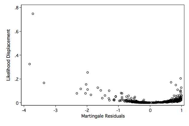
Table 6.2 on page 189 continuing to use the whas500 data. In the text, the authors highlighted points in Figures 6.4-6.8 that appeared to be points with high leverage, high influence, or large Cook’s distance. The points listed below correspond to these highlighted points.
list id bmi age hr diasbp gender chf ///
      if inlist(id,51,89,112,115,153,194,251,256,416,472), ///
      noobs sep(0)

  +----------------------------------------------------+
  |  id        bmi   age    hr   diasbp   gender   chf |
  |----------------------------------------------------|
  |  51   22.44662    80   105       72        0     1 |
  |  89   15.92695    95    62       45        0     0 |
  | 112   14.84283    87   105      104        1     0 |
  | 115   18.90242    81   118       70        1     1 |
  | 153   39.93835    32   102       83        1     0 |
  | 194   24.21079    43    47       90        0     1 |
  | 251   22.27393   102    89       60        0     1 |
  | 256   44.83886    53    96       99        1     0 |
  | 416   28.55371    80    64      198        0     0 |
  | 472   25.40431    72   186       84        0     0 |
  +----------------------------------------------------+
This set of points was arrived at using the following code to identify the highlighted observations in the figures.
* Listing of subjects identified in Figure 6.4
list id bmi scr1 if bmi < 20& scr1>8
list id bmi scr2 if bmi < 20& scr2>20
list id hr scr4 if scr4>90
list id diasbp scr5 if scr5>100

* Listing of subjects identified in Figure 6.5
list id age scr3 if age>80& scr3<-50
list id age scr8 if age>80& scr8<-150
list id chf scr7 if chf==0 & scr7>1.5
list id chf scr7 if chf==1 & scr7<-1.5
list id gender scr6 if gender==0 & scr6>1.5
list id gender scr6 if gender==1 & scr6<-1.5

* Listing of subjects identified in Figure 6.6
list id bmi db1 if bmi < 20& db1 >0.05
list id bmi db2 if bmi<20 & db2<-0.01
list id bmi db2 if bmi >41 & db2>0.01
list id hr db4 if hr>170
list id diasbp db5 if diasbp>190

* Listing of subjects identified in Figure 6.7
list id age db3 if age>85& db3<-0.002
list id age db8 if age<40 & db8 <-0.002
list id age db8 if age>70 & db8 >0.002
list id chf db7 if chf==1 & db7<-0.03
list id gender db6 if gender==0 & db6<-.15

* Listing of subjects identified in Figure 6.8
list id mgale ld if mgale<-3 &ld>.2
Table 6.3 on age 191 continuing to use the whas500 data.
stcox bmifp1 bmifp2 age hr diasbp gender chf ga if id~=416, nohr nolog

         failure _d:  fstat
   analysis time _t:  time

Cox regression -- Breslow method for ties

No. of subjects =          499                     Number of obs   =       499
No. of failures =          214
Time at risk    =  1207.671455
                                                   LR chi2(8)      =    225.90
Log likelihood  =   -1108.4149                     Prob > chi2     =    0.0000

------------------------------------------------------------------------------
          _t |      Coef.   Std. Err.      z    P>|z|     [95% Conf. Interval]
-------------+----------------------------------------------------------------
      bmifp1 |   -.685039   .1740807    -3.94   0.000    -1.026231    -.343847
      bmifp2 |   .1447858    .039543     3.66   0.000     .0672829    .2222888
         age |   .0595811    .008329     7.15   0.000     .0432565    .0759057
          hr |   .0121705   .0029455     4.13   0.000     .0063975    .0179435
      diasbp |  -.0122364   .0035128    -3.48   0.000    -.0191215   -.0053514
      gender |   1.838366   .9579476     1.92   0.055    -.0391769    3.715909
         chf |   .8302922   .1469312     5.65   0.000     .5423124    1.118272
          ga |  -.0274281   .0120524    -2.28   0.023    -.0510503   -.0038059
------------------------------------------------------------------------------
Table 6.4 on page 194 continuing to use the whas500 data. You can download stcoxgof by typing search stcoxgof and following the instructions. Slight differences in the division of the dataset into quintiles results in slight differences between the results below and the table in the text.
drop mgale

quietly stcox bmifp1 bmifp2 age hr diasbp gender chf ga if diasbp~=198, ///
     nohr nolog mgale(mgale)
stcoxgof

Goodness-of-fit test for the inclusion of design variables based on 5 quantiles of risk
(Added variables version of the Groennesby and Borgan test)

Score test                                             chi2(4)     =     9.354
                                                       Prob > chi2 =    0.0528


Likelihood-ratio test                                  LR chi2(4)  =     9.786
                                                       Prob > chi2 =    0.0442

(Table  collapsed on quantiles of linear predictor)

--------------------------------------------------------------------------------
Quantile  |
of Risk   |   Observed      Expected          z           p-Norm    Observations
----------+---------------------------------------------------------------------
        1 |         6         8.169         -.759          .448           100
        2 |        15        22.471        -1.576          .115           100
        3 |        40        37.213          .457          .648            99
        4 |        66        53.599         1.694           .09           100
        5 |        87        92.549         -.577          .564           100
          |
    Total |       214           214                                       499
--------------------------------------------------------------------------------
Table 6.5 on page 196 continuing to use the whas500 data.
drop if id==416
stcox bmifp1 bmifp2 age hr diasbp gender chf ga, nohr nolog

         failure _d:  fstat
   analysis time _t:  time

Cox regression -- Breslow method for ties

No. of subjects =          499                     Number of obs   =       499
No. of failures =          214
Time at risk    =  1207.671455
                                                   LR chi2(8)      =    225.90
Log likelihood  =   -1108.4149                     Prob > chi2     =    0.0000

------------------------------------------------------------------------------
          _t |      Coef.   Std. Err.      z    P>|z|     [95% Conf. Interval]
-------------+----------------------------------------------------------------
      bmifp1 |   -.685039   .1740807    -3.94   0.000    -1.026231    -.343847
      bmifp2 |   .1447858    .039543     3.66   0.000     .0672829    .2222888
         age |   .0595811    .008329     7.15   0.000     .0432565    .0759057
          hr |   .0121705   .0029455     4.13   0.000     .0063975    .0179435
      diasbp |  -.0122364   .0035128    -3.48   0.000    -.0191215   -.0053514
      gender |   1.838366   .9579476     1.92   0.055    -.0391769    3.715909
         chf |   .8302922   .1469312     5.65   0.000     .5423124    1.118272
          ga |  -.0274281   .0120524    -2.28   0.023    -.0510503   -.0038059
------------------------------------------------------------------------------
Table 6.6 on page 197 continuing to use the whas500 data.
lincom _b[hr]*10, hr

 ( 1)  10 hr = 0

------------------------------------------------------------------------------
          _t | Haz. Ratio   Std. Err.      z    P>|z|     [95% Conf. Interval]
-------------+----------------------------------------------------------------
         (1) |   1.129421   .0332666     4.13   0.000     1.066065    1.196541
------------------------------------------------------------------------------

lincom _b[diasbp]*10, hr

 ( 1)  10 diasbp = 0

------------------------------------------------------------------------------
          _t | Haz. Ratio   Std. Err.      z    P>|z|     [95% Conf. Interval]
-------------+----------------------------------------------------------------
         (1) |   .8848258   .0310824    -3.48   0.000     .8259553    .9478924
------------------------------------------------------------------------------

lincom _b[chf], hr

 ( 1)  chf = 0

------------------------------------------------------------------------------
          _t | Haz. Ratio   Std. Err.      z    P>|z|     [95% Conf. Interval]
-------------+----------------------------------------------------------------
         (1) |   2.293989   .3370585     5.65   0.000     1.719979    3.059563
------------------------------------------------------------------------------
Table 6.7 on page 198 continuing to use the whas500 data.
/* for coefficients */
display exp(1.838-0.027*40)

2.1340039

display exp(1.838-0.027*50)

1.6290548

display exp(1.838-0.027*60)

1.2435871

display exp(1.838-0.027*70)

.94932887

display exp(1.838-0.027*80)

.72469819

display exp(1.838-0.027*90)

.55321974

/* for confidence intervals */

lincom _b[gender]+_b[ga]*40, hr

 ( 1)  gender + 40 ga = 0

------------------------------------------------------------------------------
          _t | Haz. Ratio   Std. Err.      z    P>|z|     [95% Conf. Interval]
-------------+----------------------------------------------------------------
         (1) |   2.098539     1.0209     1.52   0.128     .8087675    5.445159
------------------------------------------------------------------------------

lincom _b[gender]+_b[ga]*50, hr

 ( 1)  gender + 50 ga = 0

------------------------------------------------------------------------------
          _t | Haz. Ratio   Std. Err.      z    P>|z|     [95% Conf. Interval]
-------------+----------------------------------------------------------------
         (1) |   1.595138   .5948045     1.25   0.210      .768064    3.312832
------------------------------------------------------------------------------

lincom _b[gender]+_b[ga]*60, hr

 ( 1)  gender + 60 ga = 0

------------------------------------------------------------------------------
          _t | Haz. Ratio   Std. Err.      z    P>|z|     [95% Conf. Interval]
-------------+----------------------------------------------------------------
         (1) |   1.212494   .3218842     0.73   0.468     .7206241    2.040095
------------------------------------------------------------------------------

lincom _b[gender]+_b[ga]*70, hr

 ( 1)  gender + 70 ga = 0

------------------------------------------------------------------------------
          _t | Haz. Ratio   Std. Err.      z    P>|z|     [95% Conf. Interval]
-------------+----------------------------------------------------------------
         (1) |   .9216391   .1621659    -0.46   0.643     .6528129    1.301167
------------------------------------------------------------------------------

lincom _b[gender]+_b[ga]*80, hr

 ( 1)  gender + 80 ga = 0

------------------------------------------------------------------------------
          _t | Haz. Ratio   Std. Err.      z    P>|z|     [95% Conf. Interval]
-------------+----------------------------------------------------------------
         (1) |   .7005548   .1002935    -2.49   0.013     .5291534    .9274761
------------------------------------------------------------------------------

lincom _b[gender]+_b[ga]*90, hr

 ( 1)  gender + 90 ga = 0

------------------------------------------------------------------------------
          _t | Haz. Ratio   Std. Err.      z    P>|z|     [95% Conf. Interval]
-------------+----------------------------------------------------------------
         (1) |   .5325046   .1052738    -3.19   0.001      .361447    .7845166
------------------------------------------------------------------------------
Figure 6.9 on page 202 continuing to use the whas500 data.
drop S0

quietly stcox bmifp1 bmifp2 age hr diasbp gender chf ga if id ~= 416, ///
      nolog nohr bases(S0)
matrix v=e(V)
generate a = bmifp1-9.9225
generate b=bmifp2-31.25588
generate ln_HR=_b[bmifp1]*a+_b[bmifp2]*b
generate HR=exp(ln_HR)
generate SE_ln_HR=sqrt(a^2*v[1,1]+b^2*v[2,2]+2*a*b*v[2,1])
generate ln_HR_l = ln_HR-1.96*SE_ln_HR
generate ln_HR_u= ln_HR+1.96*SE_ln_HR
generate HR_l=exp(ln_HR_l)
generate HR_u=exp(ln_HR_u)
generate one=1

line HR HR_l HR_u one bmi if HR_u<=10, sort clpattern(solid shortdash shortdash ".") ///
    legend(row(2) col(1) pos(12) ///
    order(1 "Estimated  Hazard Ratio" 2 "Confidence limits") ///
    ring(0) size(small)  region(lc(white))) ylabel(0 1 2 4  6 8, nogrid) ///
    ytitle("Estimated Hazard Ratio") yscale(titlegap(3))  ///
    xscale(titlegap(3) ) lc(black) graphregion(fcolor(white))
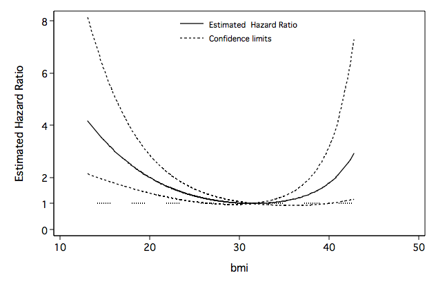
Table 6.8 on page 203 continuing to use the whas500 data.
display (15/10)^2-9.9225

-7.6725

display (15/10)^3-31.25588

-27.88088

lincom _b[bmifp1]*(-7.6725)+_b[bmifp2]*(-27.88088), hr

 ( 1) - 7.6725 bmifp1 - 27.88088 bmifp2 = 0

------------------------------------------------------------------------------
          _t | Haz. Ratio   Std. Err.      z    P>|z|     [95% Conf. Interval]
-------------+----------------------------------------------------------------
         (1) |   3.384496    .997724     4.14   0.000      1.89918    6.031451
------------------------------------------------------------------------------

display (20/10)^2-9.9225

-5.9225

display (20/10)^3-31.25588

-23.25588

lincom _b[bmifp1]*(-5.9225)+_b[bmifp2]*(-23.25588), hr

 ( 1) - 5.9225 bmifp1 - 23.25588 bmifp2 = 0

------------------------------------------------------------------------------
          _t | Haz. Ratio   Std. Err.      z    P>|z|     [95% Conf. Interval]
-------------+----------------------------------------------------------------
         (1) |   1.993758    .364173     3.78   0.000     1.393782    2.852003
------------------------------------------------------------------------------

display (25/10)^2-9.9225

-3.6725

display (25/10)^3-31.25588

-15.63088

lincom _b[bmifp1]*(-3.6725)+_b[bmifp2]*(-15.63088), hr

 ( 1) - 3.6725 bmifp1 - 15.63088 bmifp2 = 0

------------------------------------------------------------------------------
          _t | Haz. Ratio   Std. Err.      z    P>|z|     [95% Conf. Interval]
-------------+----------------------------------------------------------------
         (1) |   1.287465   .1233862     2.64   0.008     1.066988    1.553502
------------------------------------------------------------------------------

display (30/10)^2-9.9225

-.9225

display (30/10)^3-31.25588

-4.25588

lincom _b[bmifp1]*(-0.9255)+_b[bmifp2]*(-4.25588), hr

 ( 1) - .9255 bmifp1 - 4.25588 bmifp2 = 0

------------------------------------------------------------------------------
          _t | Haz. Ratio   Std. Err.      z    P>|z|     [95% Conf. Interval]
-------------+----------------------------------------------------------------
         (1) |   1.017972   .0259702     0.70   0.485      .968323    1.070167
------------------------------------------------------------------------------

display (35/10)^2-9.9225

2.3275

display (35/10)^3-31.25588
11.61912

lincom _b[bmifp1]*(2.3275)+_b[bmifp2]*(11.61912), hr

 ( 1)  2.3275 bmifp1 + 11.61912 bmifp2 = 0

------------------------------------------------------------------------------
          _t | Haz. Ratio   Std. Err.      z    P>|z|     [95% Conf. Interval]
-------------+----------------------------------------------------------------
         (1) |   1.091831   .0917488     1.05   0.296     .9260343    1.287311
------------------------------------------------------------------------------

display (40/10)^2-9.9225

6.0775

display (40/10)^3-31.25588

32.74412

lincom _b[bmifp1]*(6.0775)+_b[bmifp2]*(32.74412), hr

 ( 1)  6.0775 bmifp1 + 32.74412 bmifp2 = 0

------------------------------------------------------------------------------
          _t | Haz. Ratio   Std. Err.      z    P>|z|     [95% Conf. Interval]
-------------+----------------------------------------------------------------
         (1) |   1.781687   .5236036     1.97   0.049     1.001566    3.169445
------------------------------------------------------------------------------
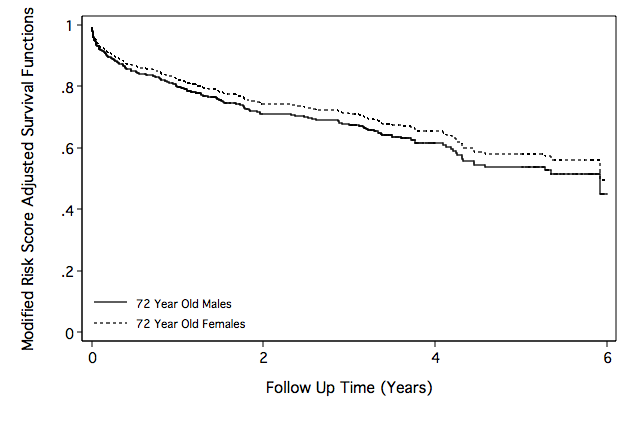
Figure 6.10 on page 204 continuing to use the whas500 data.
drop S0

quietly stcox bmifp1 bmifp2 age hr diasbp gender chf ga if id ~= 416, ///
      nolog nohr bases(S0)

predict r,xb
generate rm=r-_b[age]*age-_b[gender]*gender-_b[ga]*age*gender
quietly summarize rm, detail
display r(p50)

-1.7518661

generate S_m72=S0^(exp(r(p50)+_b[age]*72))
generate S_f72=S0^(exp(r(p50)+_b[age]*72+_b[gender]+_b[ga]*72))

line S_m72 S_f72 time if id~=416 & time < 6, c(J J) sort ///
      clpattern(solid shortdash) ///
      legend(row(2) col(1) pos(7) ///
      order(1 "72 Year Old Males" 2 "72 Year Old Females") ///
      ring(0) size(small)  region(lc(white))) ylabel(0(0.2)1, nogrid) ///
      ytitle("Modified Risk Score Adjusted Survival Functions") ///
      yscale(titlegap(3))  xscale(titlegap(3) ) ///
      lc(black) graphregion(fcolor(white)) xtitle("Follow Up Time (Years)")