Table 11.1, page 252.
use https://stats.idre.ucla.edu/stat/stata/examples/cama4/depress, clear

sort cases
by cases: tabstat sex age educat income health beddays acuteill chronill, statistics(mean sd)

_______________________________________________________________________________
-> cases = normal

   stats |       sex       age    educat    income    health   beddays  acuteill  chronill
---------+--------------------------------------------------------------------------------
    mean |  1.586066   45.2418  3.545082  21.67623  1.713115  .1721311  .2786885  .4836066
      sd |  .4935494  18.14649  1.331023  15.97547   .795869  .3782703  .4492755  .5007584
------------------------------------------------------------------------------------------

_______________________________________________________________________________
-> cases = depressed

   stats |       sex       age    educat    income    health   beddays  acuteill  chronill
---------+--------------------------------------------------------------------------------
    mean |       1.8     40.38      3.16      15.2      2.06       .42       .38       .62
      sd |   .404061  17.40032   1.16689  9.837454   .977502  .4985694  .4903144  .4903144
------------------------------------------------------------------------------------------
Figure 11.2, page 254.
NOTE: We were unable to reproduce this graph.
Table 11.2, page 255.
NOTE: You will need to download the discrim .ado and install it. You can use the search discrim command to install the program (see How can I use the search command to search for programs and get additional help? for more information about using search).
discrim cases income, predict

                   Dichotomous Discriminant Analysis

Observations    = 294                            Obs Group 0 =       244
Indep variables = 1                              Obs Group 1 =        50

Centroid 0  =   -0.0728                          R-square    =    0.0254
Centroid 1  =    0.3555                          Mahalanobis =    0.1834
Grand Cntd  =    0.2826

Eigenvalue   =    0.0261                         Wilk's Lambda =  0.9746
Canon. Corr. =    0.1594                         Chi-square    =  7.5021
Eta Squared  =    0.0254                         Sign Chi2     =  0.0062


                         Discrim Function    Unstandardized
          Variable         Coefficients        Coefficients
          -------------------------------------------------
          income              0.0283                -0.0661
          constant           -0.5223                 1.3607


                        ----- Predicted -----
            Actual   |  Group 0         Group 1 |   Total    Pr(G
            ---------+--------------------------+--------
            Group 0  |      121           123   |     244      0.83
            Group 1  |       19            31   |      50      0.17
            ---------+--------------------------+--------
            Total    |      140           154   |     294
            ---------+--------------------------+--------

                    Correctly predicted =  51.70 %
                    Model sensitivity   =  49.59 %
                    Model specificity   =  62.00 %
                    False positive      =  38.00 %
                    False negative      =  50.41 %
                    -------------------------------
                    Positive pred value =  86.43 %
                    Negative pred value =  20.13 %
                    -------------------------------
                    Kendall's tau-b     = -71.10 %
                    Cohen's kappa       =   6.34 %
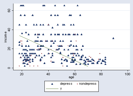
Figure 11.5, page 258.
NOTE: Please note that no carriage returns are used when issuing this command in Stata. For an explanation of the options used, please consult the Stata 8 Graphics manual.
graph scatter income age if cases==0, sym(T) || scatter income age if cases==1,sym(o) || ///
        function y = 45.089 -.622*x, range(18 70) xscale(range(15 90)) yscale(range(0 65)) ///
        xtitle(age) ytitle(income) legend(order(1 2 3) label(1 "depress") label(2 "nondepress"))
Table 11.3, page 259.
discrim cases income age, predict

                   Dichotomous Discriminant Analysis

Observations    = 294                            Obs Group 0 =       244
Indep variables = 2                              Obs Group 1 =        50

Centroid 0  =   -0.0961                          R-square    =    0.0434
Centroid 1  =    0.4690                          Mahalanobis =    0.3194
Grand Cntd  =    0.3729

Eigenvalue   =    0.0454                         Wilk's Lambda =  0.9566
Canon. Corr. =    0.2084                         Chi-square    = 12.9179
Eta Squared  =    0.0434                         Sign Chi2     =  0.0016


                         Discrim Function    Unstandardized
          Variable         Coefficients        Coefficients
          -------------------------------------------------
          income              0.0336                -0.0595
          age                 0.0209                -0.0370
          constant           -1.5157                 2.8684


                        ----- Predicted -----
            Actual   |  Group 0         Group 1 |   Total    Pr(G
            ---------+--------------------------+--------
            Group 0  |      154            90   |     244      0.83
            Group 1  |       20            30   |      50      0.17
            ---------+--------------------------+--------
            Total    |      174           120   |     294
            ---------+--------------------------+--------

                    Correctly predicted =  62.59 %
                    Model sensitivity   =  63.11 %
                    Model specificity   =  60.00 %
                    False positive      =  40.00 %
                    False negative      =  36.89 %
                    -------------------------------
                    Positive pred value =  88.51 %
                    Negative pred value =  25.00 %
                    -------------------------------
                    Kendall's tau-b     = -32.54 %
                    Cohen's kappa       =  14.85 %
Table 11.4, page 263.
NOTE: The discriminant function is given in the output above; we were unable to reproduce the classification functions.
Page 263. Covariances at the bottom of the page.
corr age income, cov

(obs=294)

             |      age   income
-------------+------------------
         age |  327.083
      income | -53.0073  233.788
Page 270. Middle of the page.
discrim cases income age
<output omitted>

display e(F)
6.6044374
NOTE: You can obtain the value of F as shown in the text by using the numbers in the output from page 259.
Page 271. Top of the page.
NOTE: The reduced model used only income, and the output from that is shown below. The rest of the numbers used in the calculations are from page 259 above.
discrim cases income
                   Dichotomous Discriminant Analysis

Observations    = 294                            Obs Group 0 =       244
Indep variables = 1                              Obs Group 1 =        50

Centroid 0  =   -0.0728                          R-square    =    0.0254
Centroid 1  =    0.3555                          Mahalanobis =    0.1834
Grand Cntd  =    0.2826

Eigenvalue   =    0.0261                         Wilk's Lambda =  0.9746
Canon. Corr. =    0.1594                         Chi-square    =  7.5021
Eta Squared  =    0.0254                         Sign Chi2     =  0.0062

                         Discrim Function    Unstandardized
          Variable         Coefficients        Coefficients
          -------------------------------------------------
          income              0.0283                -0.0661
          constant           -0.5223                 1.3607

