use https://stats.idre.ucla.edu/stat/stata/examples/chp/p157, clear
Table 6.2, page 157.
list

            t       n_t
  1.        1       355
  2.        2       211
  3.        3       197
  4.        4       166
  5.        5       142
  6.        6       106
  7.        7       104
  8.        8        60
  9.        9        56
 10.       10        38
 11.       11        36
 12.       12        32
 13.       13        21
 14.       14        19
 15.       15        15
Figure 6.5, page 159.
graph twoway scatter n_t t, ylabel(75(75)300) xlabel(3(3)15)
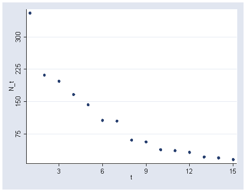
Table 6.3, page 159.
regress n_t t

  Source |       SS       df       MS                  Number of obs =      15
---------+------------------------------               F(  1,    13) =   60.62
   Model |  106080.357     1  106080.357               Prob > F      =  0.0000
Residual |  22749.3762    13  1749.95201               R-squared     =  0.8234
---------+------------------------------               Adj R-squared =  0.8098
   Total |  128829.733    14  9202.12381               Root MSE      =  41.832

------------------------------------------------------------------------------
     n_t |      Coef.   Std. Err.       t     P>|t|       [95% Conf. Interval]
---------+--------------------------------------------------------------------
       t |  -19.46429   2.499966     -7.786   0.000      -24.86513   -14.06344
   _cons |    259.581   22.72999     11.420   0.000       210.4758    308.6861
------------------------------------------------------------------------------
Figure 6.6, page 159. The rvpplot2 command can be downloaded within Stata by typing
search rvpplot2 (see How can I use
the search command to search for programs and get additional help?
for more information about using search).
rvpplot2 t, rstandard ylabel(0 1.25 2.5) xlabel(3(3)15)
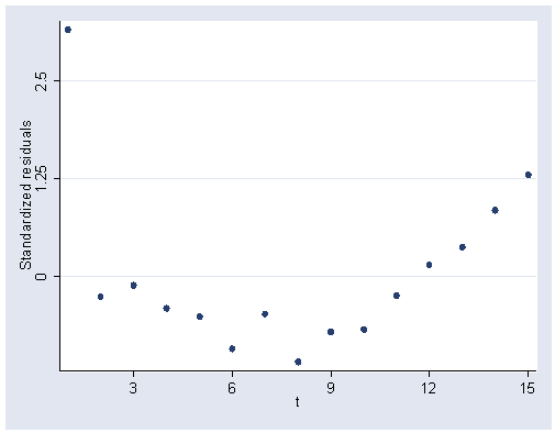
Figure 6.7, page 160.
generate lnt = log(n_t)
graph twoway scatter lnt t, ylabel(3(.75)5.25) xlabel(3(3)15)
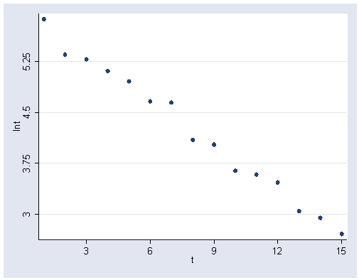
Table 6.4, page 160.
regress lnt t

  Source |       SS       df       MS                  Number of obs =      15
---------+------------------------------               F(  1,    13) = 1103.70
   Model |  13.3586861     1  13.3586861               Prob > F      =  0.0000
Residual |  .157345913    13  .012103532               R-squared     =  0.9884
---------+------------------------------               Adj R-squared =  0.9875
   Total |   13.516032    14  .965430858               Root MSE      =  .11002

------------------------------------------------------------------------------
     lnt |      Coef.   Std. Err.       t     P>|t|       [95% Conf. Interval]
---------+--------------------------------------------------------------------
       t |  -.2184253   .0065747    -33.222   0.000      -.2326291   -.2042214
   _cons |    5.97316   .0597781     99.922   0.000       5.844018    6.102303
------------------------------------------------------------------------------
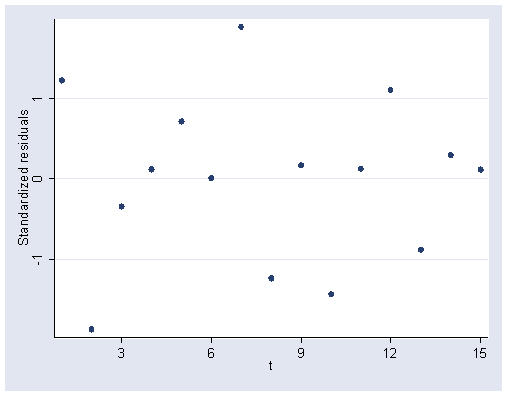
Figure 6.8, page 161.
rvpplot2 t, rstandard ylabel(-1 0 1) xlabel(3(3)15)
Input Airline Injury Data, table 6.6, page 164
Note: The input command can be used to quickly enter small datasets.
clear
input y n
11 .095
 7 .192
 7 .075
19 .2078
 9 .1382
 4 .054
 3 .1292
 1 .0503
 3 .0629
end

save airline
NOTE: Using the save command without a path specification saves
the data file in the default Stata directory, which can be seen in the lower
left corner of the Stata window.Figure 6.10, page 164
graph twoway scatter y n, ylabel(4(4)16) xlabel(.08(.04).2)
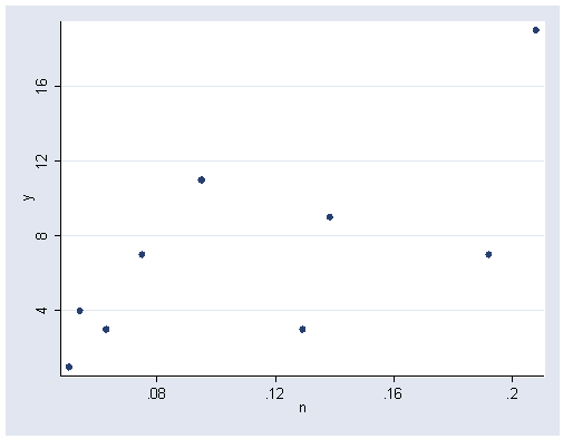
Table 6.7, page 165.
regress y n

  Source |       SS       df       MS                  Number of obs =       9
---------+------------------------------               F(  1,     7) =    6.65
   Model |  117.358709     1  117.358709               Prob > F      =  0.0365
Residual |   123.53018     7  17.6471686               R-squared     =  0.4872
---------+------------------------------               Adj R-squared =  0.4139
   Total |  240.888889     8  30.1111111               Root MSE      =  4.2009

------------------------------------------------------------------------------
       y |      Coef.   Std. Err.       t     P>|t|       [95% Conf. Interval]
---------+--------------------------------------------------------------------
       n |   64.97548   25.19587      2.579   0.037       5.396715    124.5542
   _cons |  -.1401521   3.141233     -0.045   0.966      -7.567989    7.287684
------------------------------------------------------------------------------
Figure 6.11, page 165.
rvpplot2 n, rstandard ylabel(-1 0 1) xlabel(.08(.04).2)
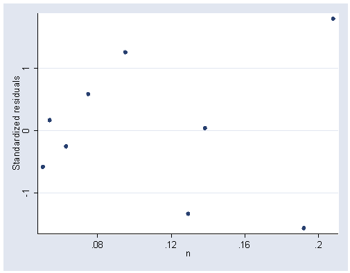
Table 6.8, page 165.
generate sqrty = sqrt(y)
(6 missing values generated)

regress sqrty n

  Source |       SS       df       MS                  Number of obs =       9
---------+------------------------------               F(  1,     7) =    6.53
   Model |  3.90772909     1  3.90772909               Prob > F      =  0.0378
Residual |  4.18610486     7   .59801498               R-squared     =  0.4828
---------+------------------------------               Adj R-squared =  0.4089
   Total |  8.09383395     8  1.01172924               Root MSE      =  .77331

------------------------------------------------------------------------------
   sqrty |      Coef.   Std. Err.       t     P>|t|       [95% Conf. Interval]
---------+--------------------------------------------------------------------
       n |   11.85643   4.638183      2.556   0.038       .8888735    22.82399
   _cons |    1.16917   .5782541      2.022   0.083       -.198184    2.536523
------------------------------------------------------------------------------
Figure 6.12, page 166.
rvpplot2 n, rstandard ylabel(-.75 0 .75) xlabel(.08(.04).2)
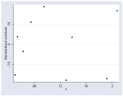
Table 6.9, page 167.
use https://stats.idre.ucla.edu/stat/stata/examples/chp/p167, clear
list

list

            x         y
  1.      294        30
  2.      247        32
  3.      267        37
  4.      358        44
  5.      423        47
..
  [remainder of output omitted]
Figure 6.13, page 167.
graph twoway scatter y x, ylabel(50(50)200) xlabel(400(400)1600)
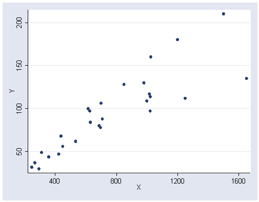
Table 6.10, page 167.
regress y x

  Source |       SS       df       MS                  Number of obs =      27
---------+------------------------------               F(  1,    25) =   86.54
   Model |  40862.6027     1  40862.6027               Prob > F      =  0.0000
Residual |   11804.064    25   472.16256               R-squared     =  0.7759
---------+------------------------------               Adj R-squared =  0.7669
   Total |  52666.6667    26  2025.64103               Root MSE      =  21.729

------------------------------------------------------------------------------
       y |      Coef.   Std. Err.       t     P>|t|       [95% Conf. Interval]
---------+--------------------------------------------------------------------
       x |   .1053611   .0113256      9.303   0.000       .0820355    .1286867
   _cons |   14.44806   9.562012      1.511   0.143      -5.245273    34.14139
------------------------------------------------------------------------------
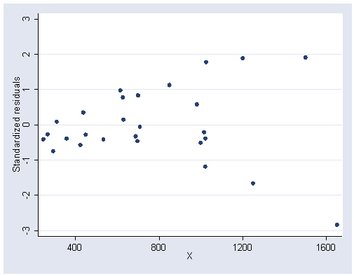
Figure 6.14, page 168.
rvpplot2 x, rstandard ylabel(-3(1)3) xlabel(400(400)1600)
Transformations of y and x, page 168.
generate ty = y/x
generate tx = 1/x
Regression used to obtain coefficients of Table 6.11, page 169.
regress ty tx

  Source |       SS       df       MS                  Number of obs =      27
---------+------------------------------               F(  1,    25) =    0.69
   Model |  .000355828     1  .000355828               Prob > F      =  0.4131
Residual |  .012842316    25  .000513693               R-squared     =  0.0270
---------+------------------------------               Adj R-squared = -0.0120
   Total |  .013198144    26  .000507621               Root MSE      =  .02266

------------------------------------------------------------------------------
      ty |      Coef.   Std. Err.       t     P>|t|       [95% Conf. Interval]
---------+--------------------------------------------------------------------
      tx |   3.803296   4.569745      0.832   0.413       -5.60827    13.21486
   _cons |   .1209903   .0089986     13.445   0.000       .1024573    .1395233
------------------------------------------------------------------------------
Figure 6.15, page 169. The rvfpplot2 command can be downloaded within Stata by typing
search rvfplot2 (see How can I use
the search command to search for programs and get additional help?
for more information about using search).
rvpplot2 tx, rstandard ylabel(-2(1)1) xlabel(.001(.001).004)
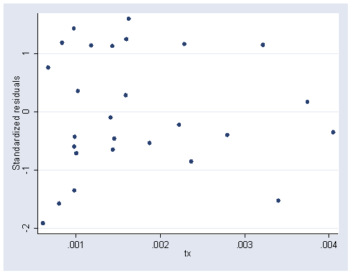
Figure 6.16, page 171.
generate lny = log(y)
graph twoway scatter lny x, ylabel(3.5(.5)5) xlabel(400(400)1600)
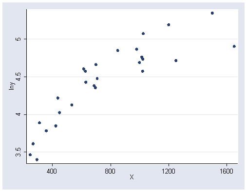
Table 6.12, page 171
regress lny x

  Source |       SS       df       MS                  Number of obs =      27
---------+------------------------------               F(  1,    25) =   83.77
   Model |  5.33672231     1  5.33672231               Prob > F      =  0.0000
Residual |  1.59258745    25  .063703498               R-squared     =  0.7702
---------+------------------------------               Adj R-squared =  0.7610
   Total |  6.92930976    26  .266511914               Root MSE      =   .2524

------------------------------------------------------------------------------
     lny |      Coef.   Std. Err.       t     P>|t|       [95% Conf. Interval]
---------+--------------------------------------------------------------------
       x |   .0012041   .0001316      9.153   0.000       .0009331     .001475
   _cons |   3.515023    .111067     31.648   0.000       3.286276     3.74377
------------------------------------------------------------------------------
Figure 6.17, page 171.
rvpplot2 x, rstandard ylabel(-3(1)1) xlabel(400(400)1600)
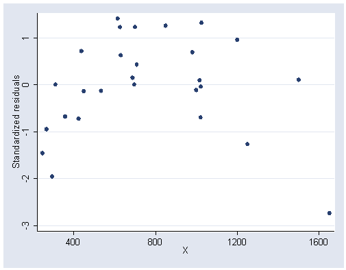
Table 6.13, page 172.
generate x2 = x^2
regress lny x x2

  Source |       SS       df       MS                  Number of obs =      27
---------+------------------------------               F(  2,    24) =   92.98
   Model |    6.137239     2   3.0686195               Prob > F      =  0.0000
Residual |  .792070761    24  .033002948               R-squared     =  0.8857
---------+------------------------------               Adj R-squared =  0.8762
   Total |  6.92930976    26  .266511914               Root MSE      =  .18167

------------------------------------------------------------------------------
     lny |      Coef.   Std. Err.       t     P>|t|       [95% Conf. Interval]
---------+--------------------------------------------------------------------
       x |   .0031127   .0003989      7.803   0.000       .0022893     .003936
      x2 |  -1.10e-06   2.24e-07     -4.925   0.000      -1.56e-06   -6.40e-07
   _cons |     2.8516   .1566401     18.205   0.000       2.528311     3.17489
------------------------------------------------------------------------------
Figure 6.18, page 172.
rvfplot2, rstandard ylabel(-1(1)2) xlabel(3.6(.4)4.8)
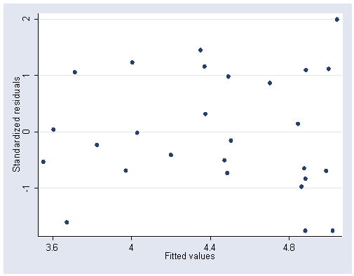
Figure 6.19, page 173.
rvpplot2 x, rstandard ylabel(-2(1)2) xlabel(400(400)1600)
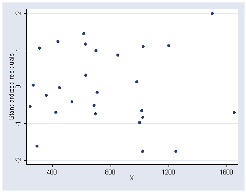
Figure 6.20, page 173.
rvpplot2 x2, rstandard ylabel(-2(1)2) xlabel(750000 2250000)
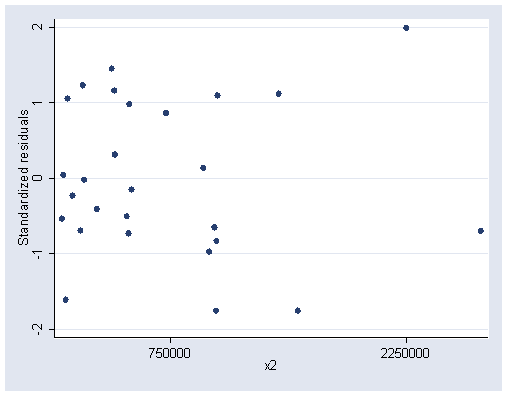
Table 6.14, page 166.
use https://stats.idre.ucla.edu/stat/stata/examples/chp/p176, clear
list

                 name   brainwei   bodyweig
  1.  Mountain beaver        8.1       1.35
  2.              Cow        423        465
  3.         Graywolf      119.5      36.33
  4.             Goat        115      27.66
  5.        Guineapig        5.5       1.04
  6.       Diplodocus         50      11700
..
  [remainder of output omitted]
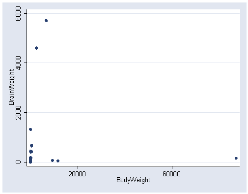
Figure 6.21, page 175.
graph twoway scatter brainwei bodyweig, xlabel(20000 60000)
Power transformations, page 175.
generate y1 = brainwei^.5
generate x1 = bodyweig^.5
generate y2 = log(brainwei)
generate x2 = log(bodyweig)
generate y3 = brainwei^-.5
generate x3 = bodyweig^-.5
generate y4 = brainwei^-1
generate x4 = bodyweig^-1
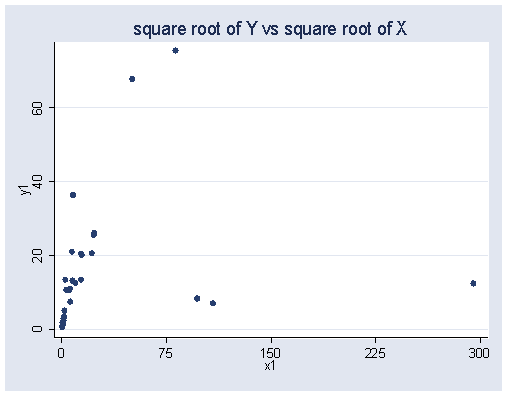
Figure 6.22, page 175.
graph twoway scatter y1 x1, ylabel(0(20)60) xlabel(0(75)300) ///
	title("square root of Y vs square root of X")
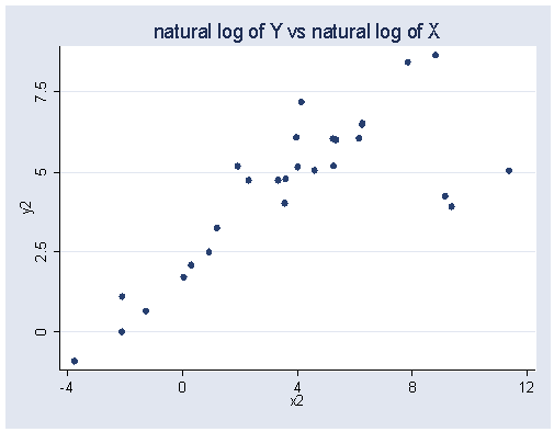
graph twoway scatter y2 x2, ylabel(0(2.5)7.5) xlabel(-4(4)12) ///
	 title("natural log of Y vs natural log of X")
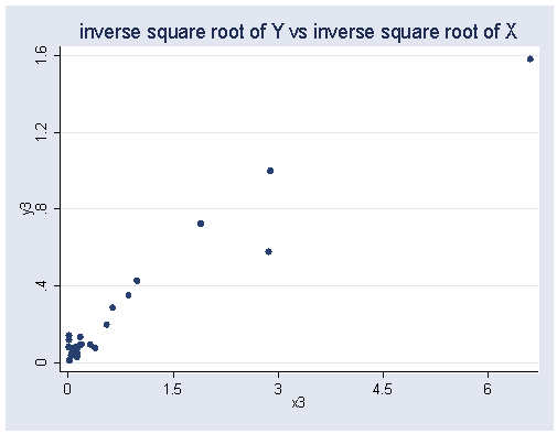
graph twoway scatter y3 x3, ylabel(0(.4)1.6) xlabel(0(1.5)6) ///
	title("inverse square root of Y vs inverse square root of X")
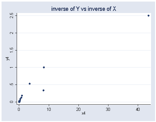
graph twoway scatter y4 x4, ylabel(0(.5)2.5) xlabel(0(10)40) ///
	title("inverse of Y vs inverse of X")